GRASS GIS 7 just got better: When reprojecting vector data, now automated vertex densification is applied. This reduces the reprojection error for long lines (or polygon boundaries). The needed improvement has been kindly added in v.proj by Markus Metz.
Example
As an (extreme?) example, we generate a box in LatLong/WGS84 (EPSG: 4326) which is of 10 degree side length (see below for screenshot and at bottom for SHAPE file download of this “box” map):
[neteler@oboe ~]$ grass70 ~/grassdata/latlong/grass7/
# for the ease of generating the box, set computational region:
g.region n=60 s=40 w=0 e=30 res=10 -p
projection: 3 (Latitude-Longitude)
zone:       0
datum:      wgs84
ellipsoid:  wgs84
north:      60N
south:      40N
west:       0
east:       30E
nsres:      10
ewres:      10
rows:       2
cols:       3
cells:      6
# generate the box according to current computational region:
v.in.region box_latlong_10deg
exit
Next we start GRASS GIS in a metric projection, here the EU LAEA:
Then we do a second reprojection with new automated vertex densification (here we use the default values for smax which is a 10km vertex distance in the reprojected map by default):
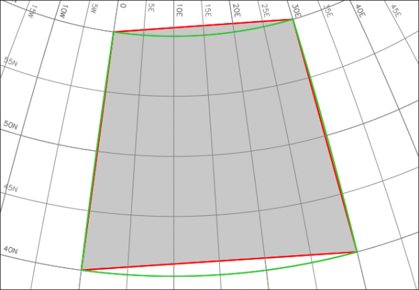
Comparison of the reprojection of a 10 degree large LatLong box to the metric EU LAEA (EPSG 3035): before in red and new in green. The grid is based on WGS84 at 5 degree spacing.
The result shows how nicely the projection is now performed in GRASS GIS 7: the red line output is old, the green color line is the new output (its area filling is not shown).
Consider to benchmark this with other GIS… the reprojected map should not become a simple trapezoid.
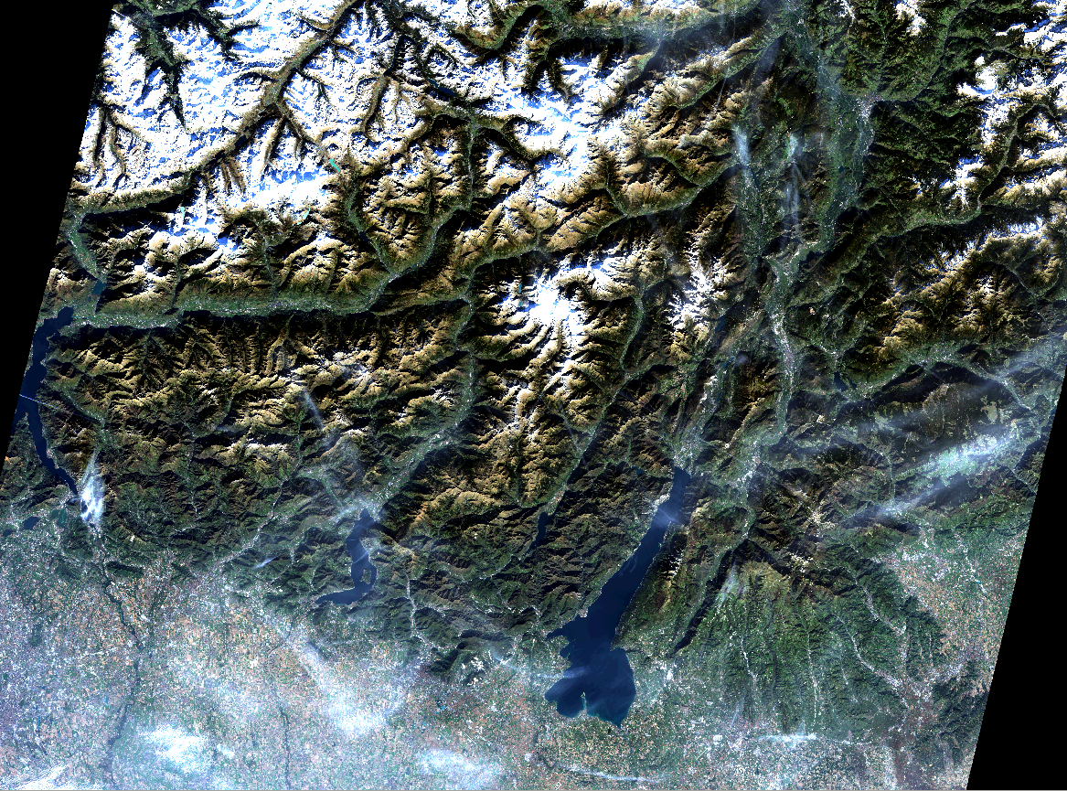
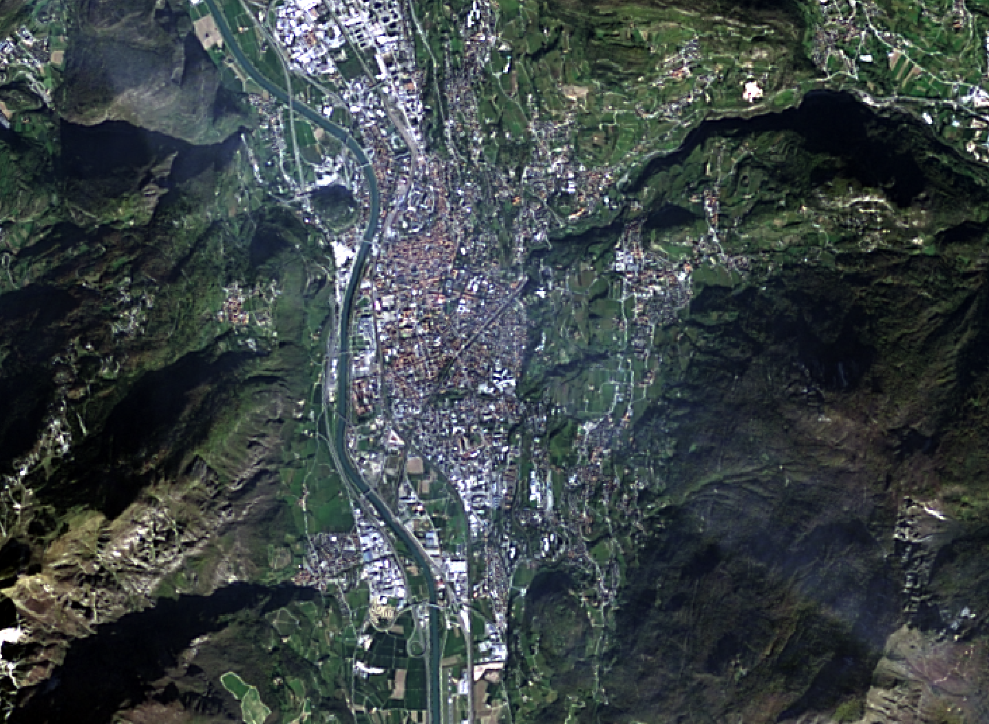
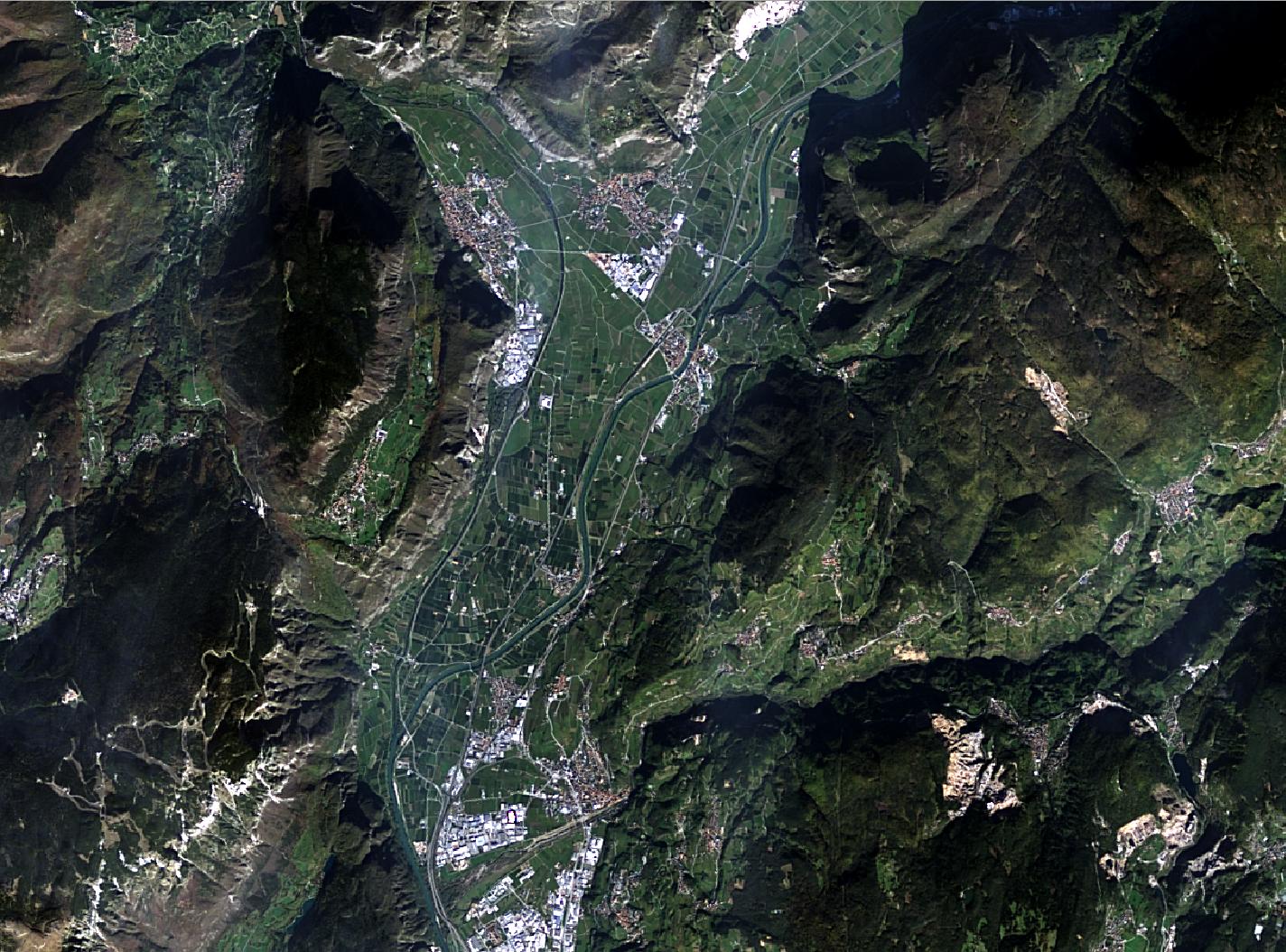
The beautiful days in early November 2014 allowed to get some nice views of the Trentino (Northern Italy) – thanks to Landsat 8 and NASA’s open data policy:
https://neteler.org/wp-content/uploads/2024/01/wg_neteler_logo.png00Markushttps://neteler.org/wp-content/uploads/2024/01/wg_neteler_logo.pngMarkus2014-11-27 18:21:412023-11-20 16:46:20Landsat 8 captures Trentino in November 2014
Do you also sometimes get maps which contain zero (0) rather than NULL (no data) in some parts of the map? This can be easily solved with “floodfilling”, even in a GIS.
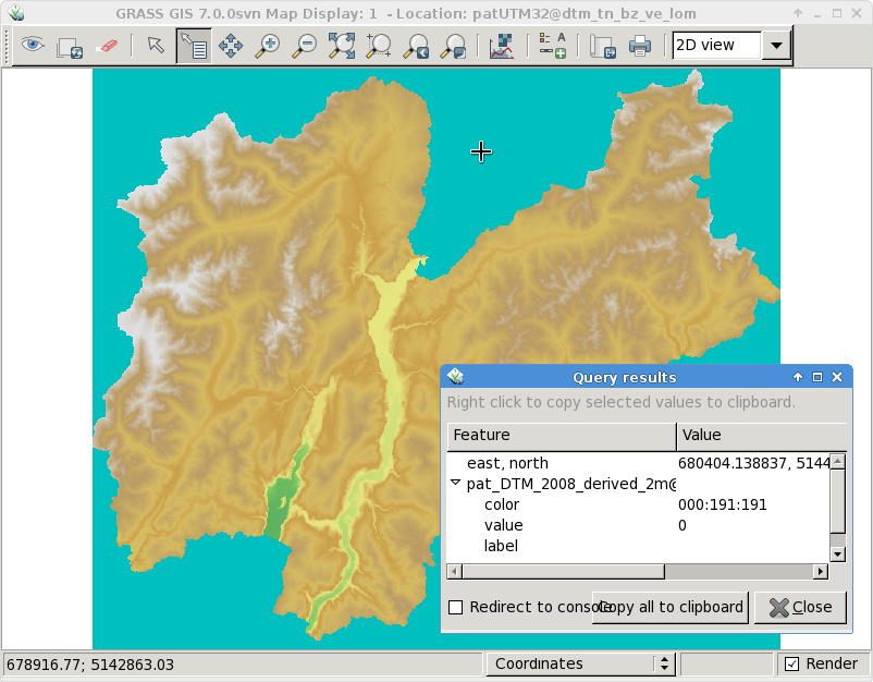
My original map looks like this (here, Trentino elevation model):
Now what? In a paint software we would simply use bucket fill but what about GIS data? Well, we can do something similar using “clumping”. It requires a bit of computational time but works perfectly, even for large DEMs, e.g., all Italy at 20m resolution. Using the open source software GRASS GIS 7, we can compute all “clumps” (that are many for a floating point DEM!):
# first we set the computational region to the raster map:
g.region rast=pat_DTM_2008_derived_2m -p
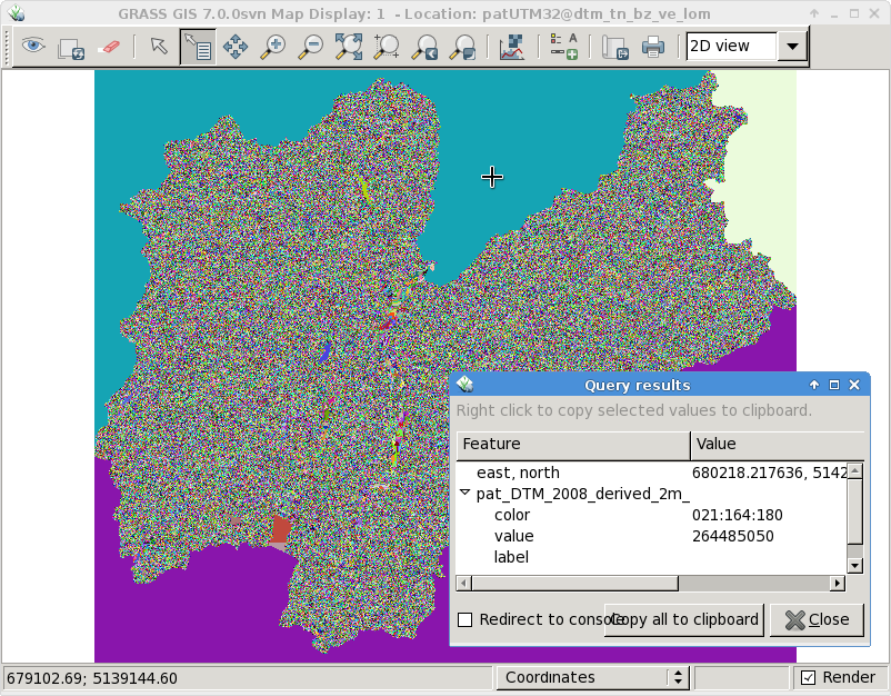
r.clump pat_DTM_2008_derived_2m out=pat_DTM_2008_derived_2m_clump
The resulting clump map produced by r.clump is nicely colorized:
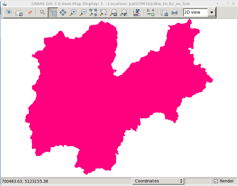
As we can see, the area of interest (province) is now surrounded by three clumps. With a simple map algebra statement (r.mapcalc or GUI calculator) we can create a MASK by assigning these outer boundary clumps to NULL and the other “good” clumps to 1:
We now activate this MASK and generate a copy of the original map into a new map name by using map algebra again (this just keeps the data matched by the MASK). Eventually we remove the MASK and verify the result:
# apply the mask
r.mask no_data_mask
# generate a copy of the DEM, filter on the fly
r.mapcalc "pat_DTM_2008_derived_2m_fixed = pat_DTM_2008_derived_2m"
# assign a nice color table
r.colors pat_DTM_2008_derived_2m_fixed color=srtmplus
# remove the MASK
r.mask -r
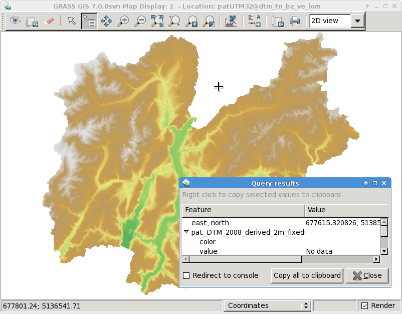
And the final DEM is now properly cleaned up in terms of NULL values (no data):
https://neteler.org/wp-content/uploads/2024/01/wg_neteler_logo.png00Markushttps://neteler.org/wp-content/uploads/2024/01/wg_neteler_logo.pngMarkus2014-09-02 20:54:412023-10-22 18:55:27Selective data removal in an elevation map by means of floodfilling
Last year (2013) I “enjoyed” a brain CT scan in order to identify a post-surgery issue – luckily nothing found. Being in Italy, like all patients I received a CD-ROM with the scan data on it: so, something to play with! In this article I’ll show how to easily turn 2D scan data into a volumetric (voxel) visualization.
First of all, we create a new XY (unprojected) GRASS location to import the data into:
# create a new, empty location (or use the Location wizard):
grass70 -c ~/grassdata/brain_ct
We now start GRASS GIS 7 with that location. After mounting the CD-ROM we navigate into the image directory therein. The directory name depends on the type of CT scanner which was used in the hospital. The file name suffix may be .IMA.
Now we count the number of images, convert and import them into GRASS GIS:
# list and count
LIST=`ls -1 *.IMA`
MAX=`echo $LIST | wc -w`
# import into XY location:
curr=1
for i in $LIST ; do
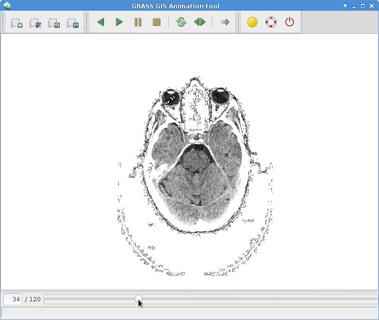
At this point all CT slices are imported in an ordered way. For extra fun, we can animate the 2D slices in g.gui.animation:
(click to enlarge)
# enter in one line:
g.gui.animation rast=`g.mlist -e rast separator=comma pattern=”brain*”`
The tool allows to export as animated GIF or AVI:
(click to enlarge)
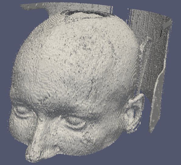
Now it is time to generate a volume:
# first count number of available layers
g.mlist rast pat=”brain*” | wc -l
# now set 3D region to number of available layers (as number of depths)
g.region rast=brain.0003 b=1 t=$MAX -p3
At this point the computational region is properly defined to our 3D raster space. Time to convert the 2D slices into voxels by stacking them on top of each other:
# convert 2D slices to 3D slices:
r.to.rast3 `g.mlist rast pat=”brain*” sep=,` out=brain_vol
We can now look at the volume with GRASS GIS’ wxNVIZ or preferably the extremely powerful Paraview. The latter requires an export of the volume to VTK format:
# fetch some environment variables
eval `g.gisenv -s`
# export GRASS voxels to VTK 3D as 3D points, with scaled z values:
SCALE=2
g.message “Exporting to VTK format, scale factor: $SCALE”
r3.out.vtk brain_vol dp=2 elevscale=$SCALE \
output=${PREFIX}_${MAPSET}_brain_vol_scaled${SCALE}.vtk -p
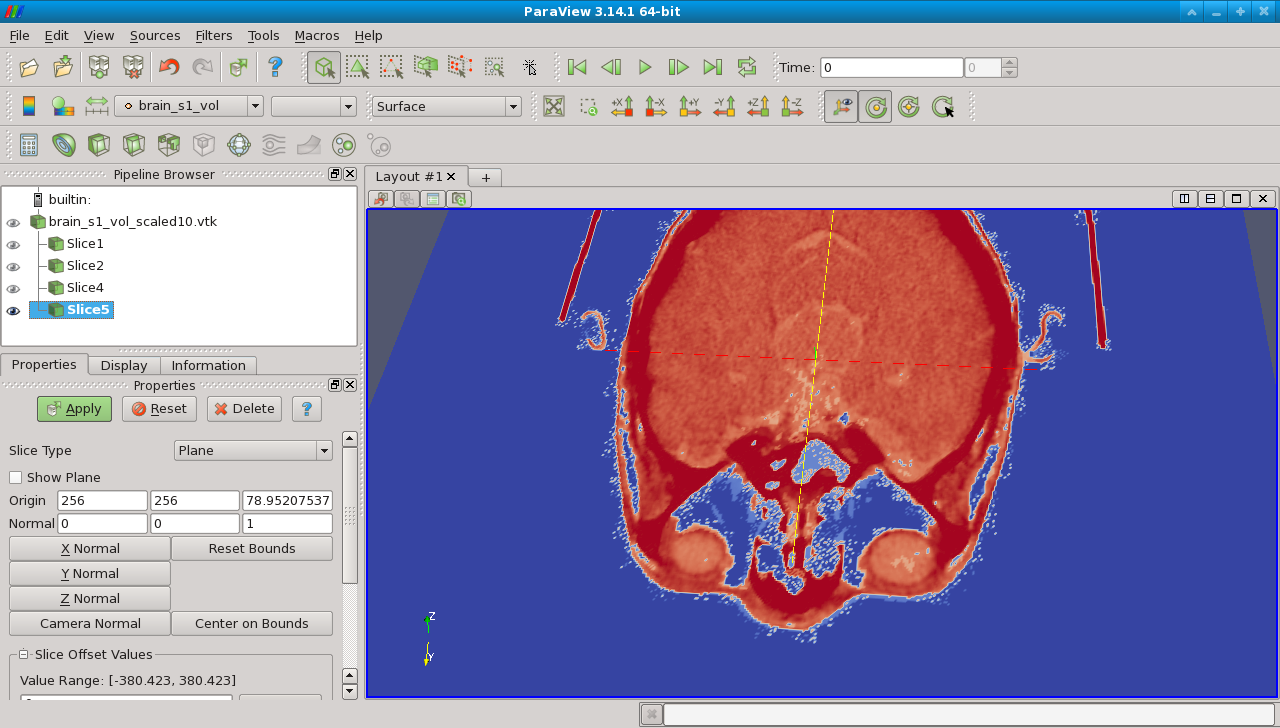
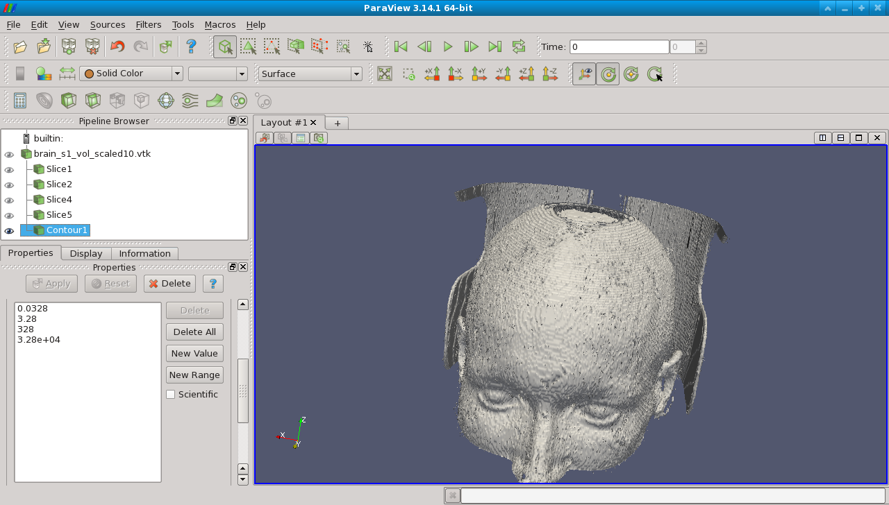
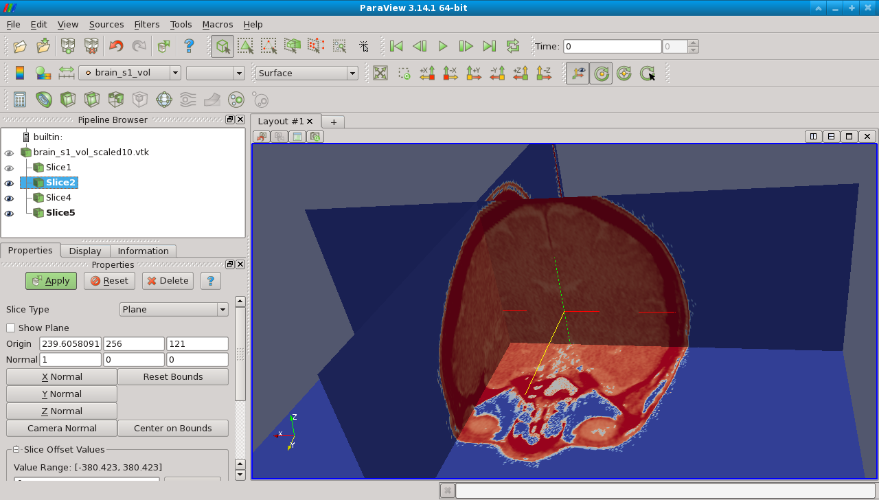
Eventually we can open this new VTK file in Paraview for visual exploration:
# show as volume
# In Paraview: Properties: Apply; Display Repres: volume; etc.
paraview –data=brain_s1_vol_scaled2.vtk
Fairly easy!
BTW: I have a scan of my non-smoker lungs as well :-)
https://neteler.org/wp-content/uploads/2024/01/wg_neteler_logo.png00Markushttps://neteler.org/wp-content/uploads/2024/01/wg_neteler_logo.pngMarkus2014-07-27 01:32:172023-10-22 18:55:21Rendering a brain CT scan in 3D with GRASS GIS 7
In order to explore all the new interfaces to PostGIS (from QGIS, GDAL, GRASS GIS 7 and others) I decided to install PostGIS 2.1 on my Fedora 20 Linux box. Eventually it is an easy job but I had to visit a series of blogs to refresh my dark memories from past PostGIS installations done some years ago… So, here the few steps:
# become root
su -
# grab the PostgreSQL 9.3 server and PostGIS 2.1
yum install postgresql-server postgresql-contrib postgis
Now the server is installed but yet inactive and not configured. The next step is to initialize, configure and start the PostgreSQL server:
# initialize DB:
postgresql-setup initdb
# start at boot time:
chkconfig postgresql on
# fire up the daemon:
service postgresql start
A test connection will show that we need to configure TCP/IP connections:
# this will fail
psql -l
psql: could not connect to server: No such file or directory
    Is the server running locally and accepting
    connections on Unix domain socket "/var/run/postgresql/.s.PGSQL.5432"?
So we enable TCP/IP connections listening on port 5432:
# edit "postgresql.conf" with editor of choice (nano, vim, ...),
# add line "listen_addresses = '*'":
vim /var/lib/pgsql/data/postgresql.conf
...
listen_addresses = '*'
#listen_addresses = 'localhost'         # what IP address(es) to listen on;
...
Now restart the PostgreSQL daemon:
# restart to re-read configuration
service postgresql restart
So far so nice. Still PostGIS is not yet active, and we need a database user “gisuser” with password:
# switch from root user to postgres user:
su - postgres
# create new DB user with password (will prompt you for it, choose a strong one):
createuser --pwprompt --encrypted gisuser
Finally we create a first database “gis”:
# create new DB
createdb --encoding=UTF8 --owner=gisuser gis
We enable it for PostGIS 2.1:
# insert PostGIS SQL magic (it should finish with a "COMMIT"):
psql -d gis -f /usr/share/pgsql/contrib/postgis-64.sql
That’s it! Now exit from the “postgres” user account a the “root” account:
# exit from PG user account (back to "root" account level):
exit
In case you want to reach the PostgreSQL/PostGIS server from outside your machine (i.e. from the network), you need to enable PostgreSQL for that:
# enable the network in pg_hba.conf (replace host line; perhaps comment IP6 line):
vim /var/lib/pgsql/data/pg_hba.conf

...
host    all             all             all                     md5
...

# save and restart the daemon:
service postgresql restart
Time for another connection test:
# we try our new DB user account on the new database (hostname is the
# name of the server in the network):
psql --user gisuser -h hostname -l
Password for user gisuser: xxxxxx
Wonderful, we are connected!
# exit from root account:
exit
[neteler@oboe ] $
Now have our PostGIS database ready!
What’s left? Get some spatial data in as a normal user:
# nice tool
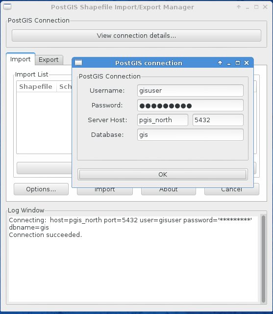
shp2pgsql-gui
Using the shp2pgsql-gui
Next pick a SHAPE file and upload it to PostGIS with “Import”.
Now connect to your PostGIS database with QGIS or GRASS GIS and enjoy!
The new version 1.11.0 of GDAL/OGR https://gdal.org/ which offers major new features has been released. GDAL/OGR is a C++ geospatial data access library for raster and vector file formats, databases and web services. It includes bindings for several languages, and a variety of command line tools.
https://neteler.org/wp-content/uploads/2024/01/wg_neteler_logo.png00Markushttps://neteler.org/wp-content/uploads/2024/01/wg_neteler_logo.pngMarkus2014-05-02 12:31:252023-11-24 23:37:31GDAL/OGR 1.11.0 released
Drowning in too many maps? Have some fun exploring fascinating geometries of changing landscapes in Space Time Cube and creating 2D and 3D animations from time series of geospatial data. Learn about the new capabilities for spatio-temporal data handling in GRASS GIS 7 (https://grass.osgeo.org/grass7/) and explore various techniques for dynamic visualizations.
First, we will introduce you to GRASS GIS 7, including its spatio-temporal capabilities and you will learn how to manage and analyze geospatial data time series. Then, we will explore new tools for visualization of spatio-temporal data. You will create both 2D and 3D dynamic visualizations directly in GRASS GIS 7. Additionally, we will explain the Space Time Cube concept using various applications based on raster and vector data time series. You will learn to manage and visualize data in space time cubes (voxel models). No prior knowledge of GRASS GIS is necessary, we will cover the basics needed for the workshop. All relevant material including an overview of the tools and hands-on practical instructions along with the sample data sets will be available on-line. And, by the way, GRASS GIS is a free and open source geographic information system (GIS) used for geospatial data management, analysis, modeling, image processing, and visualization which runs on Linux, MS Windows, Mac OS X and other systems.
Presenters: Vaclav Petras, Anna Petrasova, Helena Mitasova, Markus Neteler
When: FOSS4G 2014, Sept 8th-13th 2014, Portland, OR, USA
https://neteler.org/wp-content/uploads/2024/01/wg_neteler_logo.png00Markushttps://neteler.org/wp-content/uploads/2024/01/wg_neteler_logo.pngMarkus2014-04-12 14:30:422023-10-22 18:52:00Workshop at FOSS4G 2014: Spatio-temporal data handling and visualization in GRASS GIS 7
LiDAR point cloud data are commonly delivered in the ASPRS LAS format. The format is supported by libLAS, a BSD-licensed C++ library for reading/writing these data. GRASS GIS 7 supports the LAS format directly when built against libLAS (as the case for most binary packages being available for download).
In this exercise we will import a sample LAS data set covering a tiny area close to Raleigh, NC (USA), belonging to the North Carolina sample data set. Sample LAS data download: https://grass.osgeo.org/sampledata/north_carolina/ (25MB).
For a full exercise, we will, however, assume that no GRASS GIS location is ready so far (so: newbies are welcome!) and create a new one initially.
1. Having the LAS file: now what?
In the first place, check the metadata of the LAS file using the lasinfo command (comes with libLAS; here only parts of the output shown):
lasinfo points.las
---------------------------------------------------------
  Header Summary
---------------------------------------------------------
  Version:  1.2
  Source ID:  0
  Reserved:  0
  Project ID/GUID:  '00000000-0000-0000-0000-000000000000'
  System ID:  'libLAS'
  Generating Software:  'libLAS 1.2'
[...]
  Spatial Reference:
None
[...]
---------------------------------------------------------
  Point Inspection Summary
---------------------------------------------------------
  Header Point Count: 1287775
  Actual Point Count: 1287775

  Minimum and Maximum Attributes (min,max)
---------------------------------------------------------
  Min X, Y, Z:   6066629.86, 2190053.45, -3.60
  Max X, Y, Z:   6070237.92, 2193507.74, 906.00
  Bounding Box:  6066629.86, 2190053.45, 6070237.92, 2193507.74
  Time:  0.000000, 0.000000
  Return Number:  1, 3
  Return Count:  1, 7
  Flightline Edge:  0, 0
  Intensity:  0, 256
  Scan Direction Flag:  0, 0
  Scan Angle Rank:  0, 0
  Classification:  2, 7
  Point Source Id:  0, 0
  User Data:  0, 0
  Minimum Color (RGB):  0 0 0
  Maximum Color (RGB):  0 0 0

  Number of Points by Return
---------------------------------------------------------
  (1) 1225886  (2) 61430  (3) 459

  Number of Returns by Pulse
---------------------------------------------------------
  (1) 30877  (2) 153  (5) 1225886  (6) 30706  (7) 153

  Point Classifications
---------------------------------------------------------
  647337 Ground (2)
  639673 Low Vegetation (3)
  740 Building (6)
  25 Low Point (noise) (7)
  -------------------------------------------------------
  0 withheld
  0 keypoint
  0 synthetic
  -------------------------------------------------------
We see: no spatial reference system indicated!
Luckily we know from here that the projection is NAD83(HARN) / North Carolina, LCC 2SP metric, EPSG code 3358). Furthermore we see:
Number of Points by Return: 3 (i.e., first, mid, last)
Point Classifications: the points are already classified as “Ground” (class 2), “Low Vegetation” (3), “Building” (6), and Low Point (noise) (class 7). Something to play with later.
Time to create a GRASS GIS location and import the LAS file.
2. Creating a GRASS GIS location for the LAS file
Since we know the EPSG code of the projection, that’s an easy task. Please note that GRASS GIS can generate locations directly from SHAPE files (with .prj file), GeoTIFF and more.
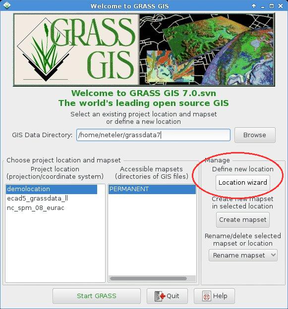
We fire up GRASS GIS 7 and open the Location Wizard:
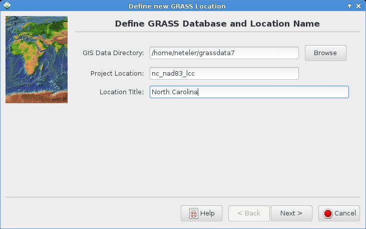
In the Location Wizard, we first define a name for the new location:
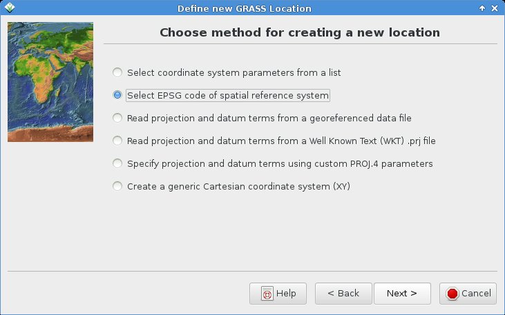
We select the “EPSG code” method for creating a new location:
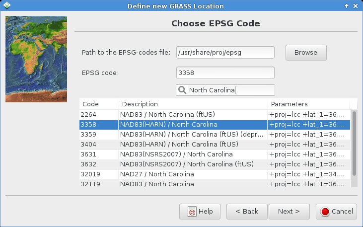
You can search for “North Carolina” and select the EPSG code 3358 from the list:
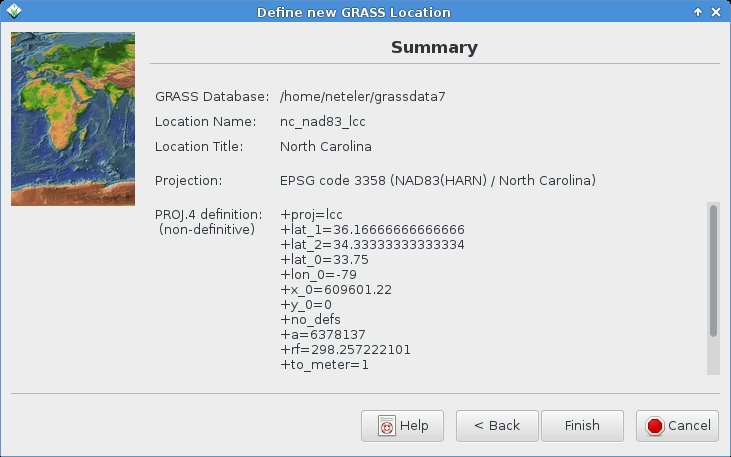
Next summary should show up as follows (be sure to have the metric projection shown!):
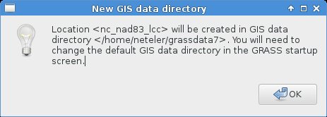
With “Finish” you reach this notification (indeed, nothing to change! It is already fine):
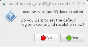
Since we want to import the LAS file, no need to manually define any region extent here – just say “No”:
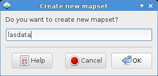
While we could import the data also into the PERMANENT mapset, we prefer to create an own mapset “lasdata” for our LAS data (once you reach hundreds of maps to manage, you will be happy about the concept of mapsets):
Voilà , we get back to the initial startup screen and can now start our GRASS GIS session with our “nc_nad83_lcc” location and “lasdata” mapset within the location: “Start GRASS”!
3. Import of the LAS file
When creating a new location from a GeoTIFF or SHAPE file (or other GDAL supported format), then the data set is imported right away. This is not the case for LAS files, also due to the fact that we can directly apply binning statistics during import of the LAS file (e.g. percentiles, min or max) and create a raster surface from the points right away rather than importing them as vector points.
3. a) Creating a raster surface from LAS during import
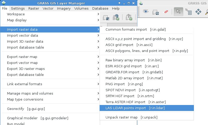
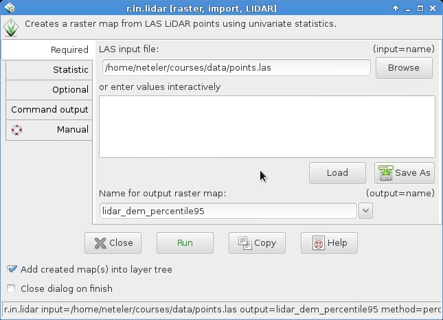
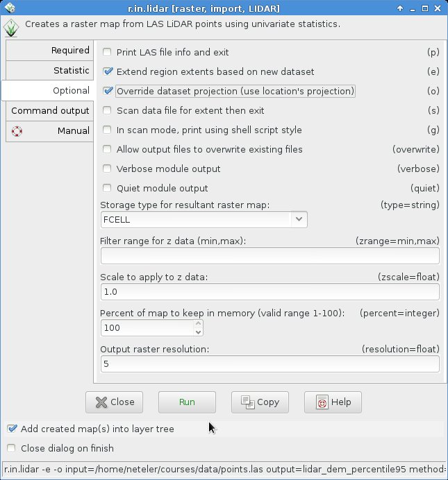
The LAS import into a raster surface is available through r.in.lidar:
First the LAS file needs to be selected and an output file name specified (in this example, we want to extract the 95th percentile as binning method, hence a reasonable map name):
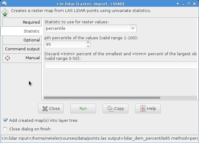
In the “Statistic” tab, we select the “percentile” method along with 95 as value:
In the “Optional” tab we activate to extend the computational region from the LAS file and, since the spatial reference system metadata are lacking from the LAS file, also “override dataset projection” to use that predefined in the location. Finally, we define 5m as desired raster resolution for the resulting raster map:
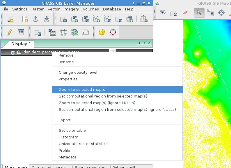
Upon conpletion of the import/binning, the new raster elevation map is shown after zooming to the map (r.in.lidar -e … restores upon completion the previous region settings, hence we may have to zoom):
Now we can start to analyze or visually explore the imported LAS file.
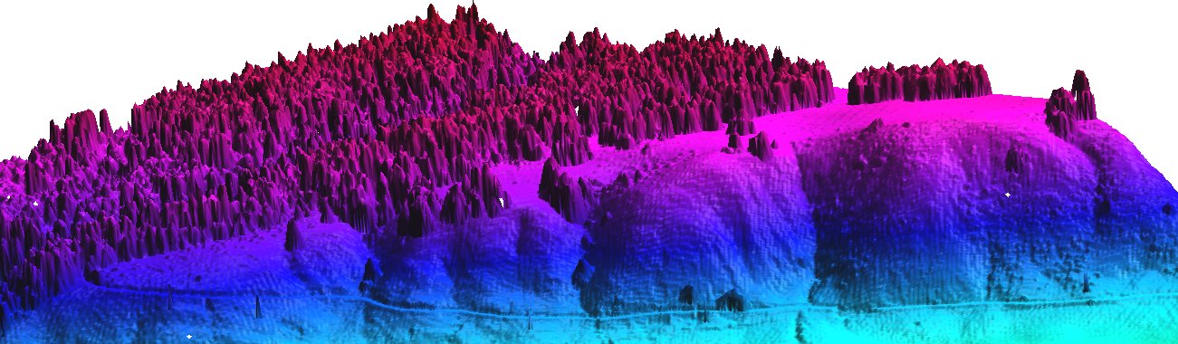
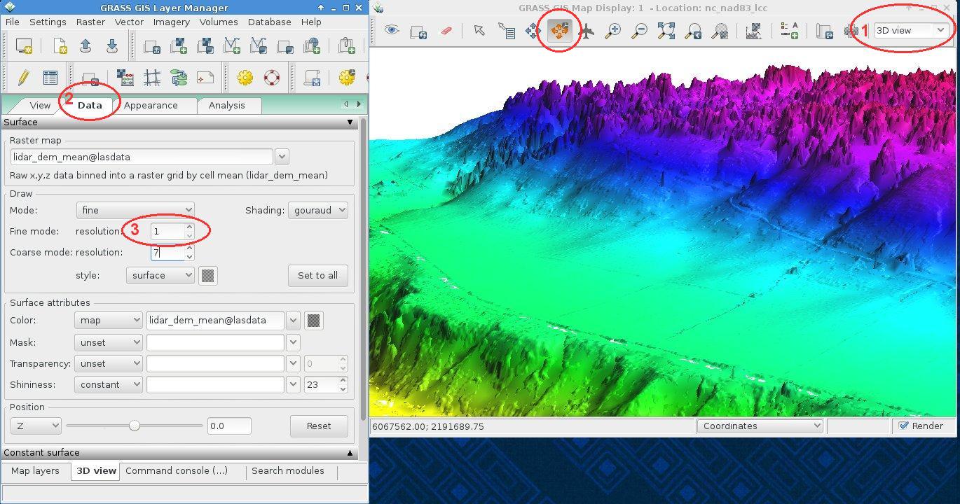
4. Visual LiDAR data exploration
Using the wxNVIZ 3D viewer, we can easily fly through the new DEM. Switch in the Map Display to “3D view” (1). Note that the default rendering is initially done at low visual resolution for speed reasons. You can switch to “Rotate mode” as well to easily navigate with the mouse. In the “Data” tab (2) you can increase the visual resolution (3) to obtain a crisp view:
https://neteler.org/wp-content/uploads/2024/01/wg_neteler_logo.png00Markushttps://neteler.org/wp-content/uploads/2024/01/wg_neteler_logo.pngMarkus2014-02-23 22:45:082023-11-20 16:35:14Importing and visualizing LAS LiDAR files in GRASS GIS 7: r.in.lidar
Recently, in order to nicely plan ahead for a birthday lunch at the agriturismo Malga Brigolina (a farm-restaurant near Sopramonte di Trento, Italy, at 1,000m a.s.l. in the Southern Alps), friends of mine asked me the day before:
“Will the place be sunny at lunch time for making a nice walk?“
[well, the weather was close to clear sky conditions but mountains are high here and cast long shadows in winter time].
A rather easy task I thought, so I got my tools ready since that was an occasion to verify the predictions with some photos! Thanks to the new EU-DEM at 25m I was able to perform the computations right away in a metric system rather than dealing with degree in LatLong.
Direct sunlight can be assessed from the beam radiation map of GRASS GIS’ r.sun when running it for a specific day and time. But even easier, there is a new Addon for GRASS GIS 7 which calculates right away time series of insolation maps given start/stop timestamps and a time step: r.sun.hourly. This shrinks the overall effort to almost nothing.
Creating the direct sunlight maps
The first step is to calculate where direct sunlight reaches the ground. Here the input elevation map is the European “eu_dem_25”, while the output is the beam radiation for a certain day (15 Dec 2013 is DOY 349).
Important hint: the computational region must be large enough to east/south/west to capure the cast shadow effects of all relevant surrounding mountains.
I let calculations start at 8am and finish at 5pm which an hourly time step. The authors have kindly parallelized r.sun.hourly, so I let it run on four processors simultaneously to speed up:
# calculate DOY (day-of-year) from given date:
date -d 2013-12-15 +%j
349

# calculate beam radiation maps for a given time period
# (note: minutes are to be given in decimal time: 30min = 0.5)
r.sun.hourly elev_in=eu_dem_25 beam_rad=trento_beam_doy349 \
      start_time=8 end_time=17 time_step=1 day=349 year=2013 \
      nprocs=4
The ten resulting maps contain the beam radiation for each pixel considering the cast shadow effects of the pixel-surrounding mountains. However, the question was not to calculate irradiance raster maps in Wh/m^2 but simply “sun-yes” or “sun-no”. So a subsequent filtering had to be applied. Each beam radiation map was filtered: if pixel value equal to 0 then “sun-no”, otherwise “sun-yes” (what my friends wanted to achieve; effectively a conversion into a binary map).
Best done in a simple shell script loop:
for map in `g.mlist rast pattern="trento_beam_doy349*"` ; do
    # rename current map to tmp
    g.rename rast=$map,$map.tmp
    # filter and save with original name
    r.mapcalc "$map = if($map.tmp == 0, null(), 1)"
    # colorize the binary map
    echo "1 yellow" | r.colors $map rules=-
    # remove cruft
    g.remove rast=$map.tmp
done
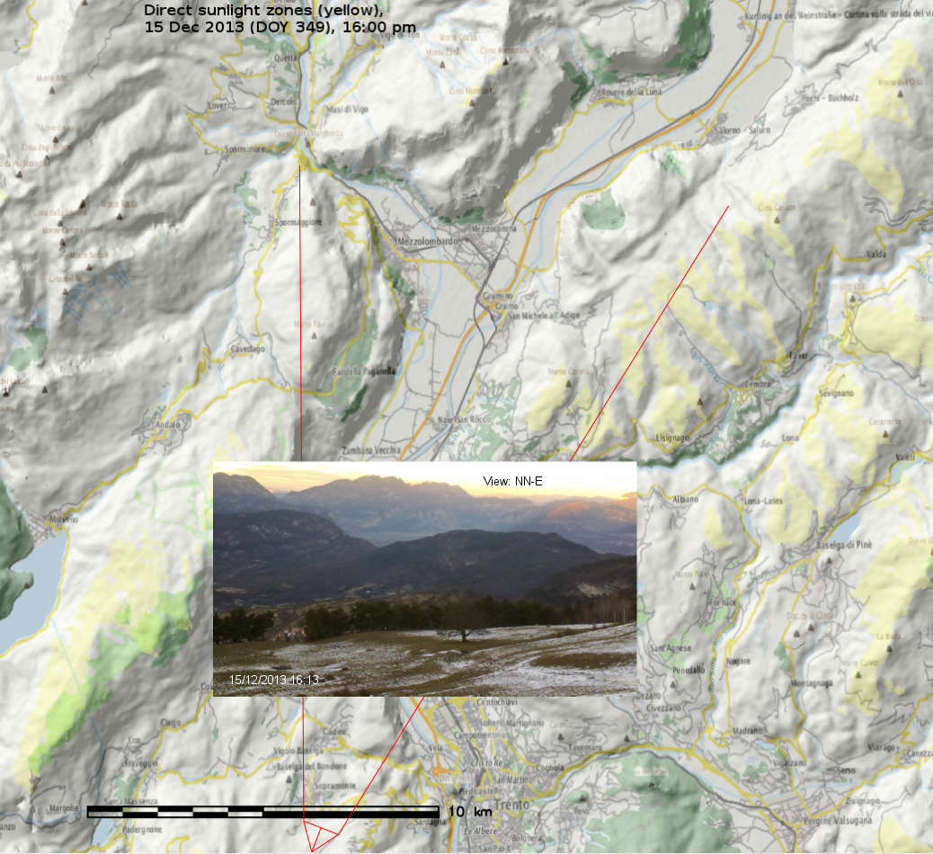
As a result we got ten binary maps, ideal for using them as overlay with shaded DEMs or OpenStreetMap layers. The areas exposed to direct sunlight are shown in yellow.
Trento, direct sunlight, 15 Dec 2013 between 10am and 5pm (See here for creating an animated GIF). Quality reduced for this blog.
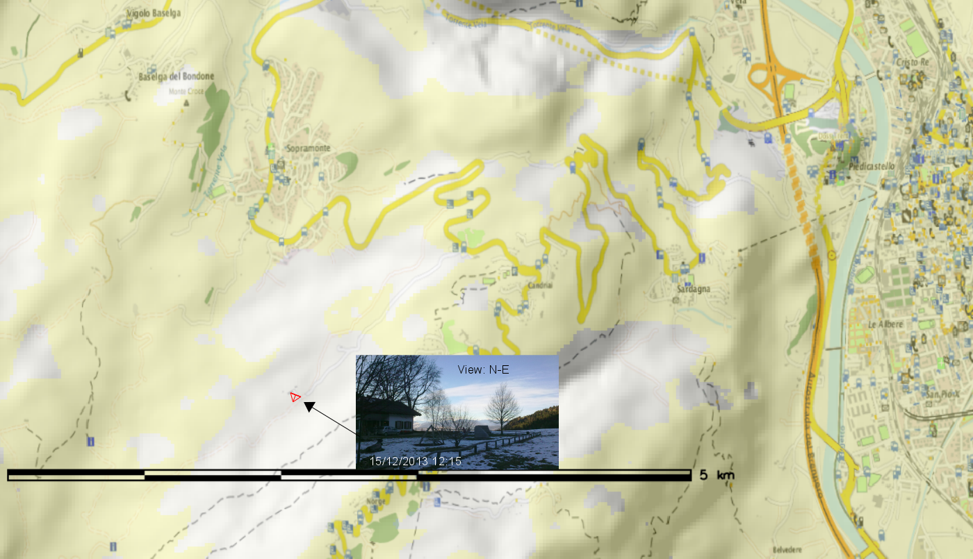
Time to look at some details: So, is Malga Brigolina in sunlight at lunch time?
Situation at 12pm (noon): predicted that the restaurant is still in shadow – confirmed in the photo:
(click to enlarge)
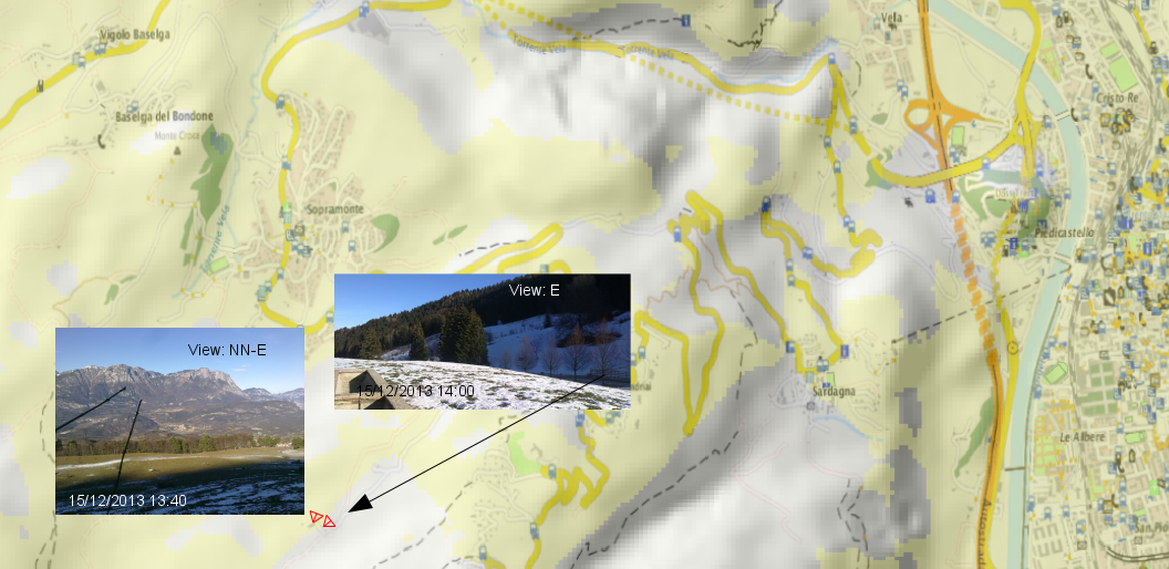
Situation at 1:30/2:00pm: sun is getting closer to the Malga, as confirmed in photo (note that the left photo is 20min ahead of the map). The small street in the right photo is still in the shadow as predicted in the map):
(click to enlarge)
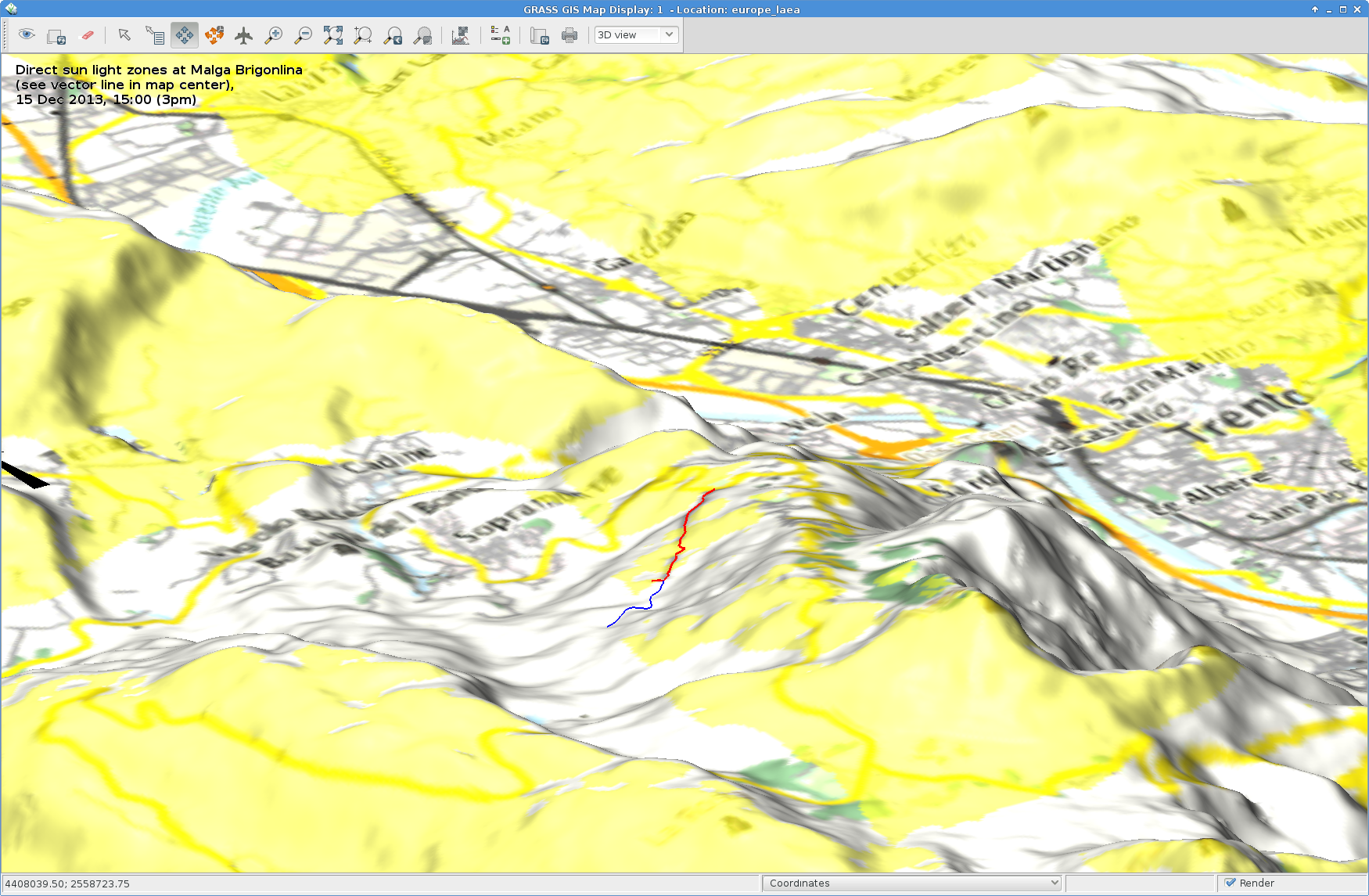
Situation at 3:00pm: sun here and there at Malga Brigolina:
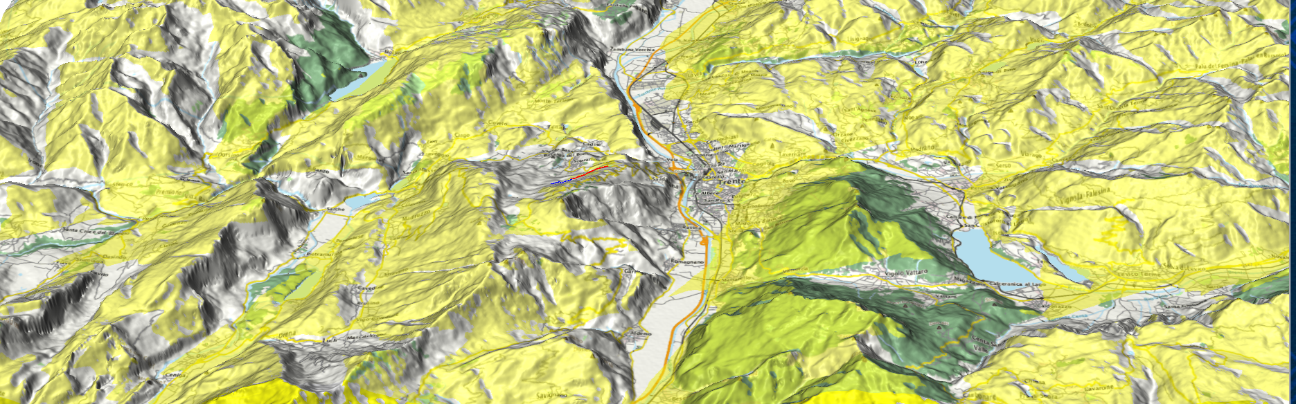
Sunlight map blended with OpenStreetmap layer (r.blend + r.composite) and draped over DEM in wxNVIZ of GRASS GIS 7 (click to enlarge). The sunday walk path around Malga Brigolina is the blue/red vector line shown in the view center.
Situation at 4:00pm: we are close to sunset in Trentino… view towards the Rotaliana (Mezzocorona, S. Michele all’Adige), last sunlit summits also seen in photo:
(click to enlarge)
Outcome
The resulting sunlight/shadow map appear to match nicely realty. Perhaps r.sun.hourly should get an additional flag to generate the binary “sun-yes” – “sun-no” maps directly.
Direct sunlight zones (yellow, 15 Dec 2013, 3pm): Trento with Monte Bondone, Paganella, Marzolan, Lago di Caldonazzo, Lago di Levico and surroundings (click to enlarge)
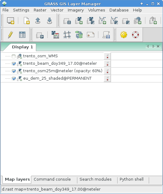
GRASS GIS usage note
The wxGUI settings were as simple as this (note the transparency values for the various layers):
https://neteler.org/wp-content/uploads/2024/01/wg_neteler_logo.png00Markushttps://neteler.org/wp-content/uploads/2024/01/wg_neteler_logo.pngMarkus2013-12-27 21:52:402023-11-20 10:13:45Will the sun shine on us?