The EuroLST dataset is seamless and gap-free with a temporal resolution of four records per day and enhanced spatial resolution of 250 m. This newly developed reconstruction method (Metz et al, 2014) has been applied to Europe and neighbouring countries, resulting in complete daily coverage from 2001 onwards. To our knowledge, this new reconstructed LST time series exceeds the level of detail of comparable reconstructed LST datasets by several orders of magnitude. Studies on emerging diseases, parasite risk assessment and temperature anomalies can now be performed on the continental scale, maintaining high spatial and temporal detail. In their paper, the authors provide examples for implications and applications of the new LST dataset, such as disease risk assessment, epidemiology, environmental monitoring, and temperature anomalies.
Reconstructed MODIS Land Surface Temperature Dataset, at 250m pixel resolution (click figure to enlarge):
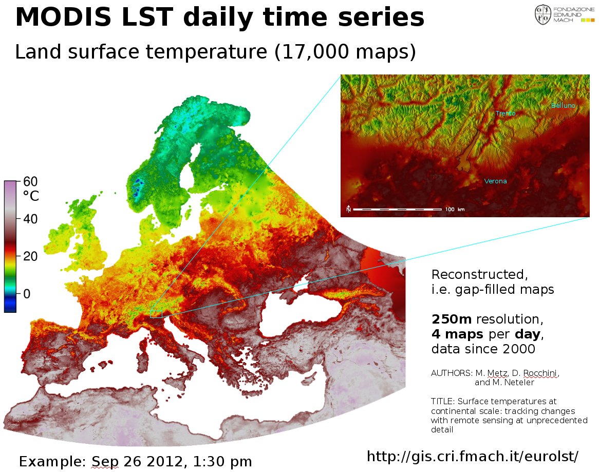
MODIS Land Surface Temperature (LST) reconstructed (gap-filled)
Article and data citation:
EuroLST has been produced by the former PGIS group at Fondazione Edmund Mach, DBEM based on daily MODIS LST (Product of NASA) maps.
Metz, M.; Rocchini, D.; Neteler, M. 2014: Surface temperatures at the continental scale: Tracking changes with remote sensing at unprecedented detail. Remote Sensing. 2014, 6(5): 3822-3840 (DOI | HTML | PDF)
Used software
Open Source commands used in processing (GRASS GIS 7):
links to the related manual pages involved in the data preparation
- i.pca: Principal Components Analysis (PCA) for image processing.
- r.regression.multi: it calculates multiple linear regression from raster maps
- v.surf.bspline: it performs bicubic or bilinear spline interpolation with Tykhonov regularization.
Furthermore:
- r.bioclim: calculates various bioclimatic indices from monthly temperature and optional precipitation time series (install in GRASS GIS 7 with “g.extention r.bioclim”)
- pyModis: Free and Open Source Python based library to work with MODIS data
Metadata
Map projection: EPSG 3035, prj file
PROJCS["Lambert Azimuthal Equal Area",
    GEOGCS["grs80",
        DATUM["European_Terrestrial_Reference_System_1989",
            SPHEROID["Geodetic_Reference_System_1980",6378137,298.257222101]],
        PRIMEM["Greenwich",0],
        UNIT["degree",0.0174532925199433]],
    PROJECTION["Lambert_Azimuthal_Equal_Area"],
    PARAMETER["latitude_of_center",52],
    PARAMETER["longitude_of_center",10],
    PARAMETER["false_easting",4321000],
    PARAMETER["false_northing",3210000],
    UNIT["Meter",1]]
Selected open data derived from EuroLST
BIOCLIM derived from reconstructed MODIS LST at 250m pixel resolution


BIOCLIM-like European LST maps following the “Bioclim” definition (Hutchinson et al., 2009) – derived from 10 years of reconstructed MODIS LST (download to be completed) as GeoTIFF files, 250m pixel resolution, in EU LAEA projection:
- BIO1: Annual mean temperature (°C*10): eurolst_clim.bio01.zip (MD5) 72MB
- BIO2: Mean diurnal range (Mean monthly (max – min tem)): eurolst_clim.bio02.zip (MD5) 72MB
- BIO3: Isothermality ((bio2/bio7)*100): eurolst_clim.bio03.zip (MD5) 72MB
- BIO4: Temperature seasonality (standard deviation * 100): eurolst_clim.bio04.zip (MD5) 160MB
- BIO5: Maximum temperature of the warmest month (°C*10): eurolst_clim.bio05.zip (MD5) 106MB
- BIO6: Minimum temperature of the coldest month (°C*10): eurolst_clim.bio06.zip (MD5) 104MB
- BIO7: Temperature annual range (bio5 – bio6) (°C*10): eurolst_clim.bio07.zip (MD5) 132MB
- BIO10: Mean temperature of the warmest quarter (°C*10): eurolst_clim.bio10.zip (MD5) 77MB
- BIO11: Mean temperature of the coldest quarter (°C*10): eurolst_clim.bio11.zip (MD5) 78MB
Each ZIP file contains the respective GeoTIFF file (for cell value units, see below), the color table as separate ASCII file and a README.txt with details.
WMS/WCS Server
Using this URL, you can read the EuroLST BIOCLIM data directly via OGC WMS and WCS protocol:
https://web.archive.org/web/20220615191155/https://geodati.fmach.it/production/ows_europe_lst
OpenData License
The data published in this page are open data and released under the ODbL (Open Database License).
The full EuroLST dataset is not released online as open data (size: 18TB), please ask Luca Delucchi or Roberto Zorer for more info
Acknowledgments
The MOD11A1.005, MYD11A1.005 were retrieved from the online web site, courtesy of the NASA EOSDIS Land Processes Distributed Active Archive Center (LP DAAC), USGS/Earth Resources Observation and Science (EROS) Center, Sioux Falls, South Dakota, https://e4ftl01.cr.usgs.gov/