[toc]

Recently, in order to nicely plan ahead for a birthday lunch at the agriturismo Malga Brigolina (a farm-restaurant near Sopramonte di Trento, Italy, at 1,000m a.s.l. in the Southern Alps), friends of mine asked me the day before:

Will the place be sunny at lunch time for making a nice walk?

[well, the weather was close to clear sky conditions but mountains are high here and cast long shadows in winter time].

paganella_rotaliana

A rather easy task I thought, so I got my tools ready since that was an occasion to verify the predictions with some photos! Thanks to the new EU-DEM at 25m I was able to perform the computations right away in a metric system rather than dealing with degree in LatLong.

Direct sunlight can be assessed from the beam radiation map of GRASS GIS’ r.sun when running it for a specific day and time. But even easier, there is a new Addon for GRASS GIS 7 which calculates right away time series of insolation maps given start/stop timestamps and a time step: r.sun.hourly. This shrinks the overall effort to almost nothing.

Creating the direct sunlight maps

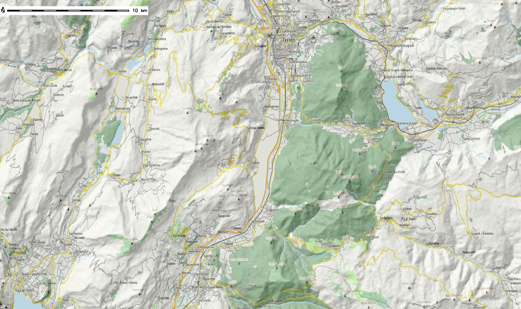
The first step is to calculate where direct sunlight reaches the ground. Here the input elevation map is the European “eu_dem_25”, while the output is the beam radiation for a certain day (15 Dec 2013 is DOY 349).

Important hint: the computational region must be large enough to east/south/west to capure the cast shadow effects of all relevant surrounding mountains.

I let calculations start at 8am and finish at 5pm which an hourly time step. The authors have kindly parallelized r.sun.hourly, so I let it run on four processors simultaneously to speed up:

# calculate DOY (day-of-year) from given date:
date -d 2013-12-15 +%j
349

# calculate beam radiation maps for a given time period
# (note: minutes are to be given in decimal time: 30min = 0.5)
r.sun.hourly elev_in=eu_dem_25 beam_rad=trento_beam_doy349 \
      start_time=8 end_time=17 time_step=1 day=349 year=2013 \
      nprocs=4

The ten resulting maps contain the beam radiation for each pixel considering the cast shadow effects of the pixel-surrounding mountains. However, the question was not to calculate irradiance raster maps in Wh/m^2 but simply “sun-yes” or “sun-no”. So a subsequent filtering had to be applied. Each beam radiation map was filtered: if pixel value equal to 0 then “sun-no”, otherwise “sun-yes” (what my friends wanted to achieve; effectively a conversion into a binary map).
Best done in a simple shell script loop:

[Edit 30 Dec 2013: thanks to Anna you can simplify below loop to the r.colors call thanks to the new -b flag for binary output in r.sun.hourly!]

for map in `g.mlist rast pattern="trento_beam_doy349*"` ; do
    # rename current map to tmp
    g.rename rast=$map,$map.tmp
    # filter and save with original name
    r.mapcalc "$map = if($map.tmp == 0, null(), 1)"
    # colorize the binary map
    echo "1 yellow" | r.colors $map rules=-
    # remove cruft
    g.remove rast=$map.tmp
done

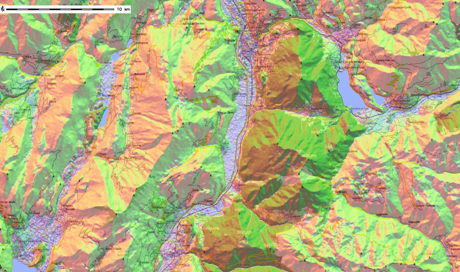
As a result we got ten binary maps, ideal for using them as overlay with shaded DEMs or OpenStreetMap layers. The areas exposed to direct sunlight are shown in yellow.

Trento direct sunlight 15 Dec 2013 Animation

Trento, direct sunlight, 15 Dec 2013 between 10am and 5pm (See here for creating an animated GIF). Quality reduced for this blog.

Time to look at some details: So, is Malga Brigolina in sunlight at lunch time?

Situation at 12pm (noon): predicted that the restaurant is still in shadow – confirmed in the photo:
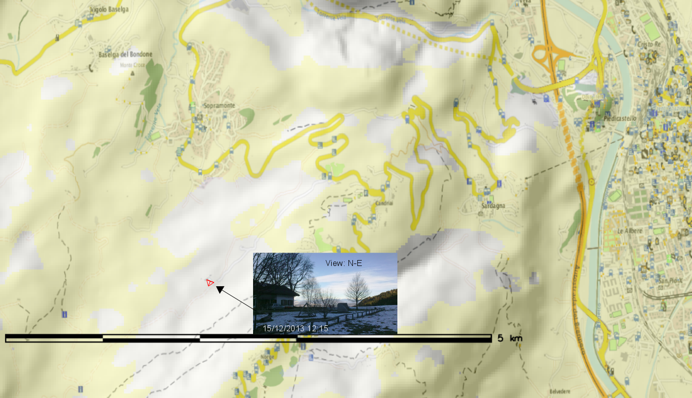
malga_brigolina_direct_sunlight_15dec2013_12pm_foto

(click to enlarge)

Situation at 1:30/2:00pm: sun is getting closer to the Malga, as confirmed in photo (note that the left photo is 20min ahead of the map). The small street in the right photo is still in the shadow as predicted in the map):
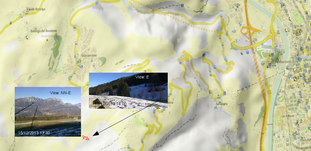
malga_brigolina_direct_sunlight_15dec2013_14pm_foto(click to enlarge)

Situation at 3:00pm: sun here and there at Malga Brigolina:

malga_brigolina_direct_sunlight_15dec2013_15pm_3D
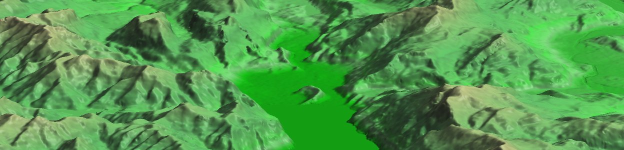
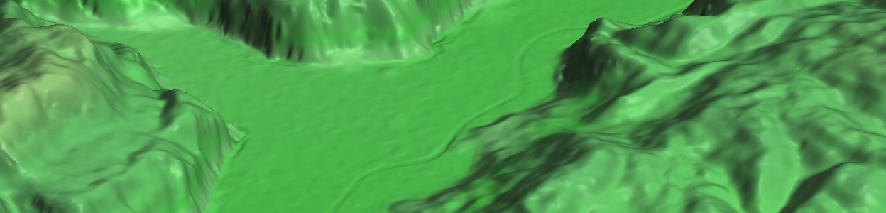
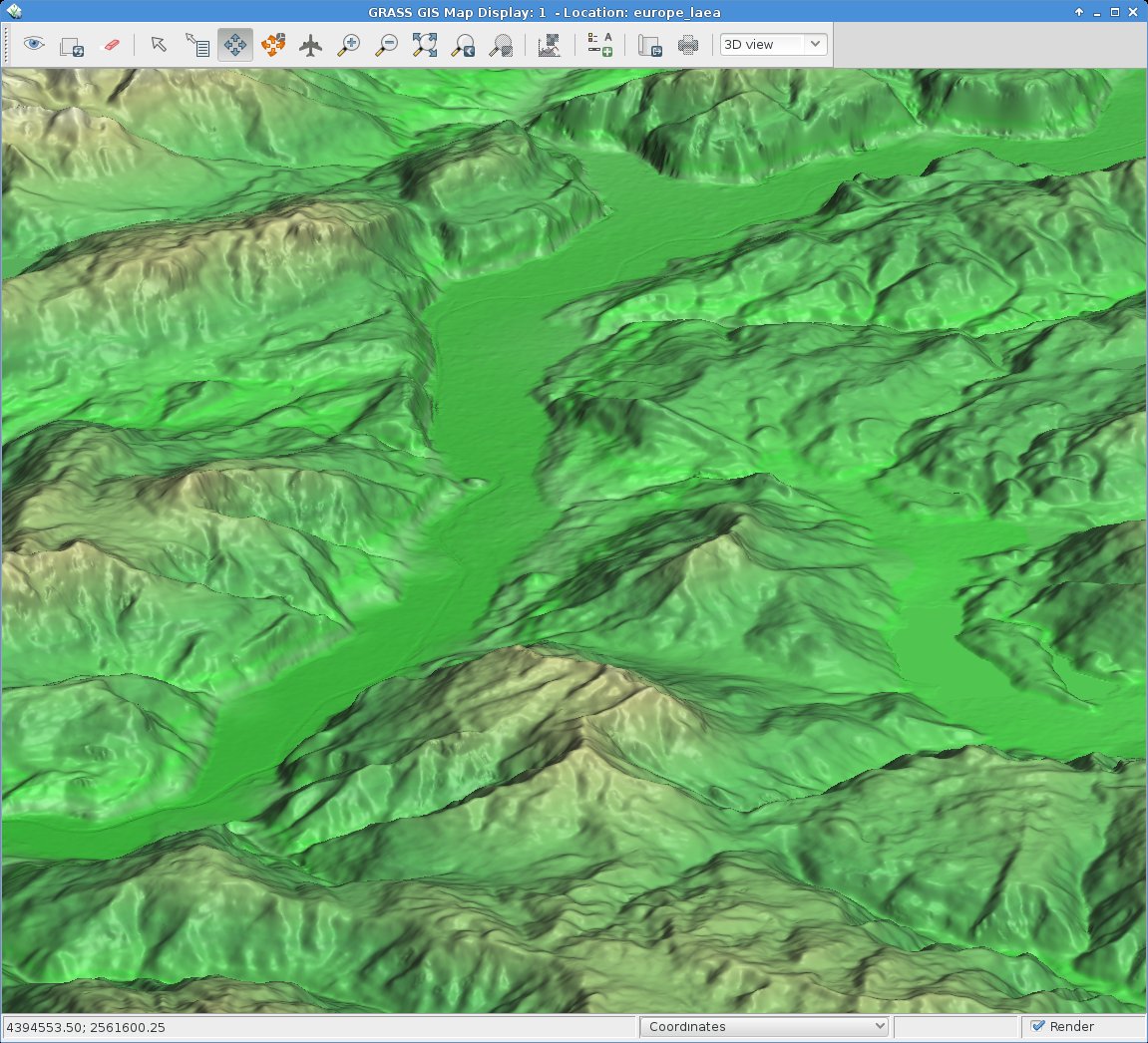
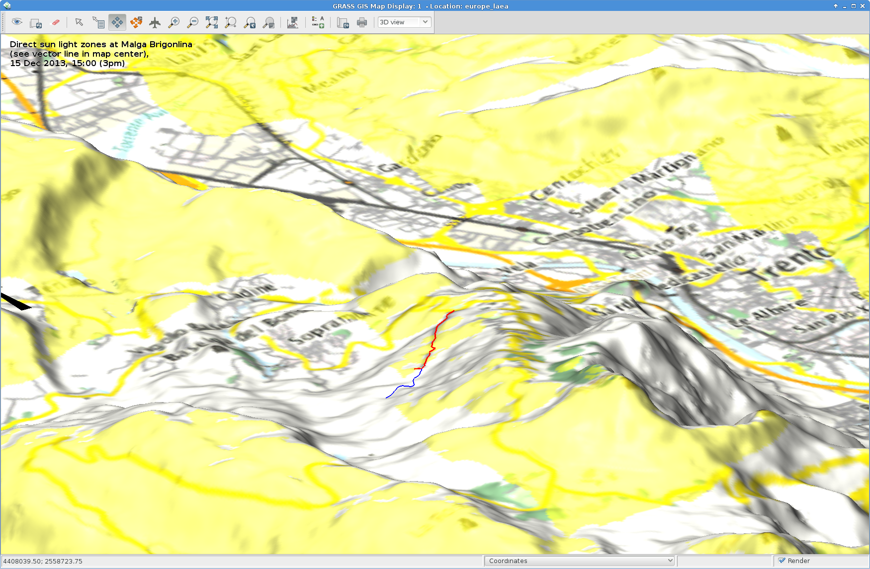
Sunlight map blended with OpenStreetmap layer (r.blend + r.composite) and draped over DEM in wxNVIZ of GRASS GIS 7 (click to enlarge). The sunday walk path around Malga Brigolina is the blue/red vector line shown in the view center.

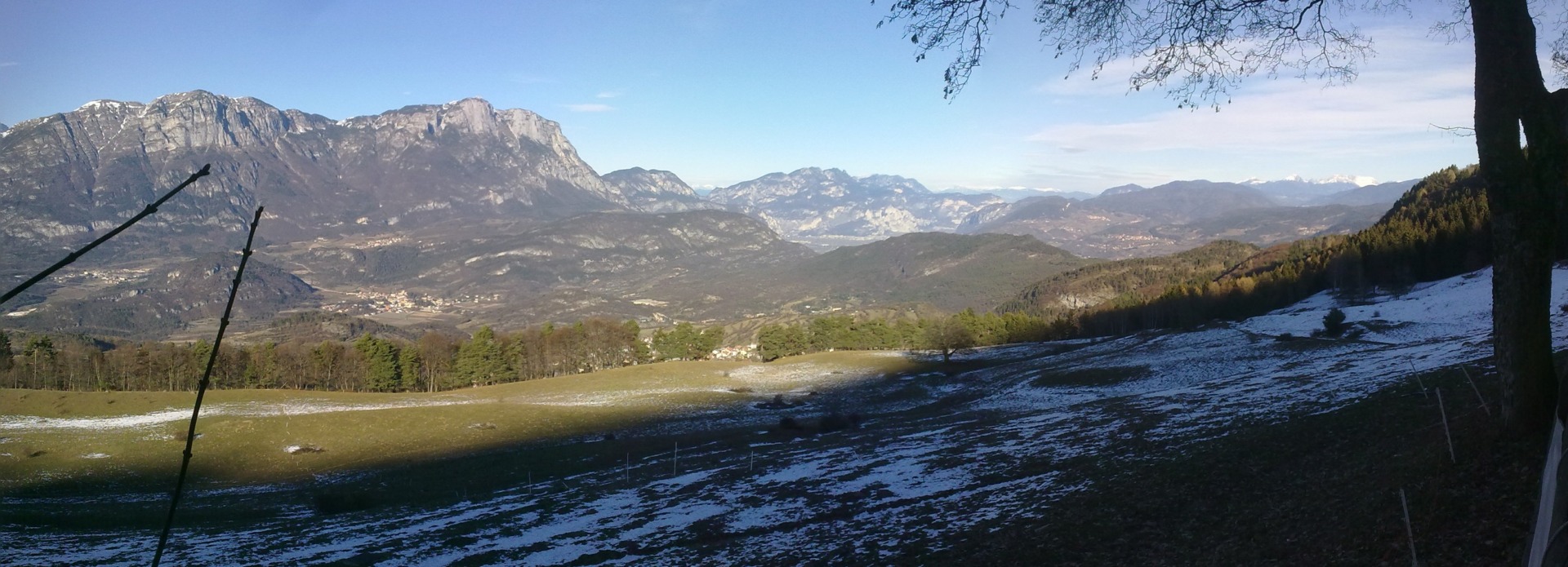
Situation at 4:00pm: we are close to sunset in Trentino… view towards the Rotaliana (Mezzocorona, S. Michele all’Adige), last sunlit summits also seen in photo:
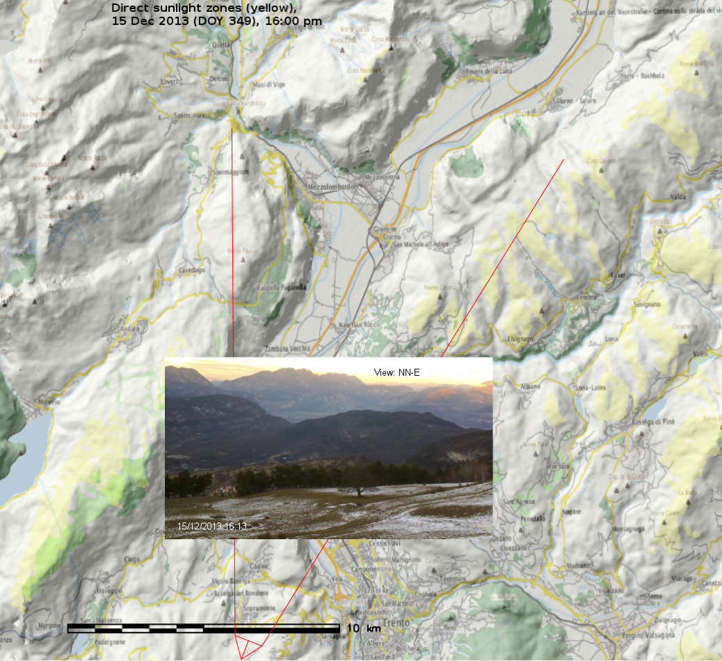
rotaliana_direct_sunlight_15dec2013_16pm_foto(click to enlarge)

Outcome

The resulting sunlight/shadow map appear to match nicely realty. Perhaps r.sun.hourly should get an additional flag to generate the binary “sun-yes” – “sun-no” maps directly.

trento_direct_sunlight_15dec2013_15pm_3D
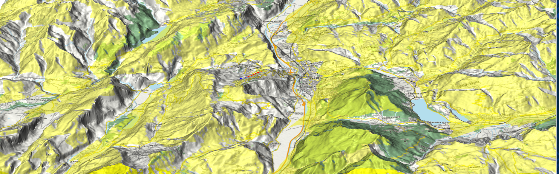
Direct sunlight zones (yellow, 15 Dec 2013, 3pm): Trento with Monte Bondone, Paganella, Marzolan, Lago di Caldonazzo, Lago di Levico and surroundings (click to enlarge)

GRASS GIS usage note

The wxGUI settings were as simple as this (note the transparency values for the various layers):
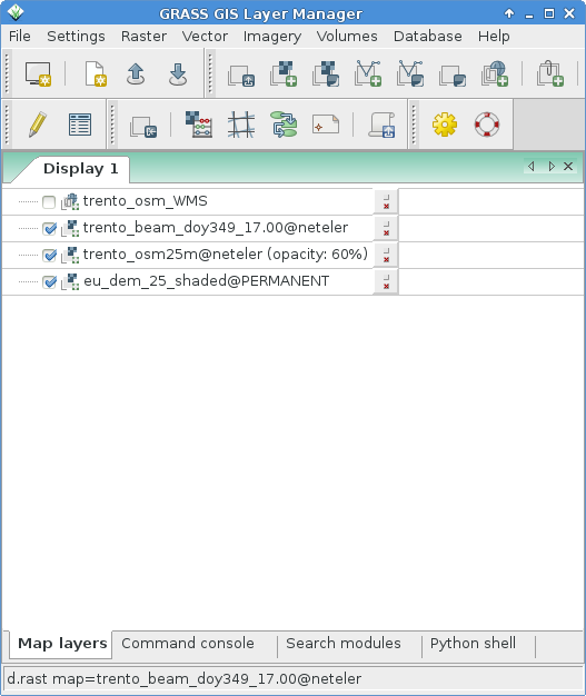
trento_direct_sunlight_wxGUI

Data sources:

Lorem ipsum dolor sit amet, consectetuer adipiscing elit. Aenean commodo ligula eget dolor. Aenean massa. Cum sociis natoque penatibus et magnis dis parturient montes, nascetur ridiculus mus. Donec quam felis, ultricies nec, pellentesque eu, pretium quis, sem. Nulla consequat massa quis enim. Donec pede justo, fringilla vel, aliquet nec, vulputate eget, arcu. In enim justo, rhoncus ut, imperdiet a, venenatis vitae, justo.

Nullam dictum felis eu pede mollis pretium. Integer tincidunt. Cras dapibus. Vivamus elementum semper nisi. Aenean vulputate eleifend tellus. Aenean leo ligula, porttitor eu, consequat vitae, eleifend ac, enim. Aliquam lorem ante, dapibus in, viverra quis, feugiat a, tellus.


Read more

Watch how the community based GRASS GIS 6.4 software development evolved! You can see how the individual contributors modify and expand the source code – click screenshot for Youtube video:

GRASS GIS 6.4 development visualization from 1999 to 2013 (with soundtrack)

  • Dec 29, 1999: GRASS GIS 5.0 is being stored in an online source code repository in December 1999…
  • Dec 02, 2000: The developers work on all parts of the code…
  • Jan 15, 2002: Working on the future GRASS GIS 5.1 release
  • Nov 25, 2002: Starting GRASS 5.1 development with code restructuring
  • Jun 14, 2004: GRASS GIS 5.7 released in June 2004
  • Nov 09, 2004: Source code restructuring to get a better directory layout (all other developers waiting…)
  • Nov 09, 2004: … thousands of files are modified in this operation …
  • Nov 10, 2004: All developers resume their activities after the restructuring
  • Jan 10, 2005: Preparing the GRASS GIS 6.0.0 release…
  • Apr 09, 2005: GRASS GIS 6.0.0 published, release branch being split off from trunk for easier maintenance
  • Feb 22, 2006: Release of GRASS GIS 6.0.2 and new source code refactoring startedApr 05, 2006: Heavy development activity in trunk (development branch) …
  • Oct 25, 2006: GRASS GIS 6.2.0 released in October 2006
  • Apr 10, 2007: Preparing the GRASS GIS 6.2.2 release…
  • Jun 16, 2007: GRASS GIS 6.2.2 released in June 2007
  • Nov 01, 2007: Raster and vector modules being actively maintained…
  • Apr 02, 2007: New graphical user interface development speeding up (wxGUI)
  • Feb 20, 2008: Copyright statements prettified in many files
  • May 31, 2008: New GRASS 6 development branch being split off from trunk (which becomes GRASS 7)
  • Jun 10, 2008: Developers moving over to new branch
  • Feb 23, 2009: GRASS 6.4 release branch split off from GRASS 6 development branch
  • Apr 03, 2009: GRASS GIS 6.4 preparations starting…
  • Feb 24, 2010: Intense maintenance in GRASS 6.4 release branch
  • Sep 15, 2010: GRASS GIS 6.4.0 released in September 2010
  • Apr 12, 2011: GRASS GIS 6.4.1 released in April 2011
  • Jun 27, 2011: GRASS GIS 6.4.svn matures for the upcoming 6.4.2 release
  • Aug 16, 2011: Intense maintenance in GRASS 6.4 release branch (GRASS GIS 7 development not shown here)…
  • Feb 19, 2012: GRASS GIS 6.4.2 released in February 2012
  • Nov 13, 2012: Backporting graphical user interface bugfixes from GRASS GIS 7 to GRASS GIS 6.4
  • Apr 17, 2013: Further maintenance in GRASS 6.4 release branch
  • Jul 10, 2013: Fixing odds ‘n ends for the new stable release
  • Jul 27, 2013: GRASS GIS 6.4.3 released in July 2013

The corresponding timeline is also available at
https://grass.osgeo.org/home/history/releases/

THANKS TO ALL CONTRIBUTORS!
https://grass.osgeo.org/development/

Rendering: Markus Neteler
Audio track editing: Duccio Rocchini & Antonio Galea

Music:
Le bruit peut rendre sourd – Track 6/18 Album “Sensation electronique” by Saelynh (CC-BY-NC-ND) https://www.jamendo.com/en/track/1236/le-bruit-peut-rendre-sourd

Software used:
Gource software: https://code.google.com/p/gource/ (GPL)
OpenShot video editor: https://www.openshotvideo.com/ (GPL

Inspired by Vaclav Petras posting about “Did you know that you can see streets of downtown Raleigh in elevation data from NC sample dataset?” I wanted to try the new GRASS GIS 7 Addon r.shaded.pca which creates shades from various directions and combines then into RGB composites just to see what happens when using the new EU-DEM at 25m.

To warm up, I registered the “normally” shaded DEM (previously generated with gdaldem) with r.external in a GRASS GIS 7 location (EPSG 3035, LAEA) and overlayed the OpenStreetMap layer using WMS with GRASS 7’s r.in.wms. An easy task thanks to University of Heidelberg’s www.osm-wms.de. Indeed, they offer a similar shading via WMS, however, in the screenshot below you see the new EU data being used for controlling the light on our own:

OpenStreetMap shaded with EU DEM 25m

OpenStreetMap shaded with EU DEM 25m (click to enlarge)

Next item: trying r.shaded.pca… It supports multi-core calculation and the possibility to strengthen the effects through z-rescaling. In my example, I used:

r.shaded.pca input=eu_dem_25 output=eu_dem_25_shaded_pca nproc=3 zmult=50

The leads to a colorized hillshading map, again with the OSM data on top (50% transparency):

eu_dem_25m_PCA_shaded_OSM_trento_rovereto_garda_lake

OpenStreetMap shaded with r.shaded.pca using EU DEM 25m (click to enlarge)

Yes, fun – I like it :-)

Data sources:

eu_dem_upper_garda_lake_riva_arco_italy

EU DEM 25m upper Garda Lake area with Riva del Garda and Arco (Italy). 3D view in wxNVIZ – GRASS GIS 7

The 25m European Digital Elevation Model (EU-DEM, Version 1) is a Digital Surface Model (DSM) representing the first surface as illuminated by the sensors:

eu_dem_s_michele_rotaliana_italy

EU DEM Rotaliana with Mezzocorona and S. Michele (Italy). Produced using Copernicus data and information funded by the European Union – EU-DEM layers.

Its elevations were captured at 1 arc second postings (2.78E-4 degrees). The tiles are provided at 25m resolution in EU-LAEA (EPSG. 3035) projection, temporal coverage: 2000, published in Oct 2013. It is a realisation of the Copernicus programme, managed by the European Commission, DG Enterprise and Industry. Metadata are provided here. According to their “Methodology” page it is a hybrid product based on SRTM and ASTER GDEM data fused by a weighted averaging approach and it has been generated as a contiguous dataset divided into 1 degree by 1 degree tiles, corresponding to the SRTM naming convention. In addition to the DEM data, a colour shaded relief image over Europe is provided.

From the metadata page: “The EU-DEM data are provided as is, i.e. without a formal validation yet. An independent statistical validation is scheduled as part of the GIO land monitoring service activities, and will be made available in the course of 2014.

Data download

Note that the GeoTIFF files are of major size, up to 5 GB:

Data import

The data come as ZIP compressed files, hence unzipping occurs (or simply use the fancy “vsizip” driver in GDAL).

Hint for GRASS GIS users: instead of importing the data, you can use the r.external command to register the GeoTIFF DEM file instead of imorting it within a EU LAEA projected location.

Enjoy!

eu_dem_trento_adige_s_michele_italy