[toc]

The Landsat 8 mission is a collaboration between the U.S. Geological Survey (USGS) and National Aeronautics and Space Administration (NASA) which continues the acquisition of high-quality data for observing land use and land cover change.

The Landsat 8 spacecraft which was launched in 2013 carries they following key instruments:

• OLI: the Operational Land Imager which collects data in the visible, near infrared, and shortwave infrared wavelength regions as well as a panchromatic band. With respect to Landsat 7 two new spectral bands have been added: a deep-blue band for coastal water and aerosol studies (band 1), and a band for cirrus cloud detection (band 9). Furthermore, a Quality Assurance band (BQA) is also included to indicate the presence of terrain shadowing, data artifacts, and clouds.
• TIRS: The Thermal Infrared Sensor continues thermal imaging and is also intended to support emerging applications such as modeling evapotranspiration for monitoring water use consumption over irrigated lands.

The data from Landsat 8 are available for download at no charge and with no user restrictions.

For our analysis example, we’ll obtain (freely – thanks to NASA and USGS!) a Landsat 8 scene from https://earthexplorer.usgs.gov/

First of all, you should register.

Landsat 8 download procedure

1. Enter Search Criteria:

• path/row tab, enter Type WRS2: Path: 16, Row: 35
• Date range: 01/01/2013 – today
• Click on the “Data sets >>” button

2. Select Your Data Set(s):

• Expand the entry + Landsat Archive
  [x] L8 OLI/TIRS
• Click on the “Results >>” button

(We jump over the additional criteria)

4. Search Results

From the resulting list, we pick the data set:

Entity ID: LC80160352013134LGN03
Coordinates: 36.04321,-79.28696
Acquisition Date: 14-MAY-13

Using the “Download options”, you can download the data set (requires login). Select the choice:
[x] Level 1 GeoTIFF Data Product (842.4 MB)

You will receive the file “LC80160352013134LGN03.tar.gz”.

Unpacking the downloaded Landsat 8 dataset

To unpack the data, run (or use a graphical tool at your choice):

tar xvfz LC80160352013134LGN03.tar.gz

A series of GeoTIFF files will be extracted: LC80160352013134LGN03_B1.TIF, LC80160352013134LGN03_B2.TIF, LC80160352013134LGN03_B3.TIF, LC80160352013134LGN03_B4.TIF, LC80160352013134LGN03_B5.TIF, LC80160352013134LGN03_B6.TIF, LC80160352013134LGN03_B7.TIF, LC80160352013134LGN03_B8.TIF, LC80160352013134LGN03_B9.TIF, LC80160352013134LGN03_B10.TIF, LC80160352013134LGN03_B11.TIF, LC80160352013134LGN03_BQA.TIF

We may check the metadata with “gdalinfo“:

gdalinfo LC80160352013134LGN03_B1.TIF
Driver: GTiff/GeoTIFF
Files: LC80160352013134LGN03_B1.TIF
Size is 7531, 7331
Coordinate System is:
PROJCS["WGS 84 / UTM zone 17N",
  GEOGCS["WGS 84",
  DATUM["WGS_1984",
  SPHEROID["WGS 84",6378137,298.257223563,
...
Pixel Size = (30.000000000000000,-30.000000000000000)
...

Want to spatially subset the Landsat scene first?

If you prefer to cut out a smaller area (subregion), check here for gdal_translate usage examples.

Import into GRASS GIS 7

Note: While this Landsat 8 scene covers the area of the North Carolina (NC) sample dataset, it is delivered in UTM rather than the NC’s state plane metric projection. Hence we preprocess the data first in its original UTM projection prior to the reprojection to NC SPM.

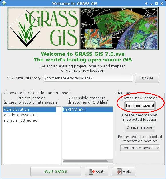
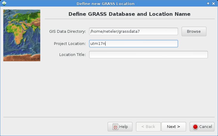
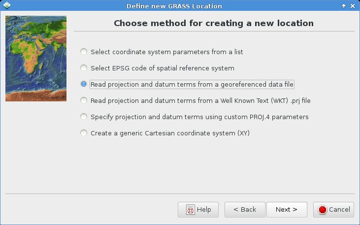
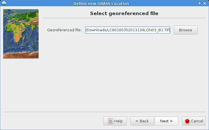
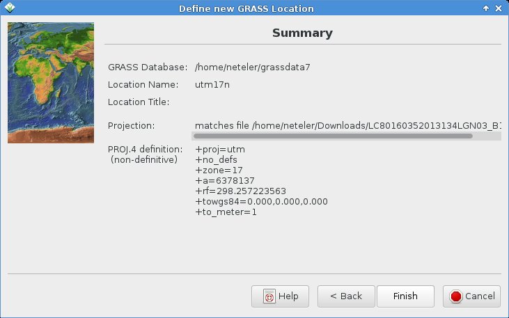
Using the Location Wizard, we can import the dataset easily into a new location (in case you don’t have UTM17N not already created earlier):

grass70 -gui

 

 

 

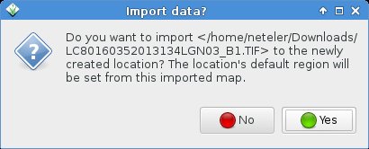
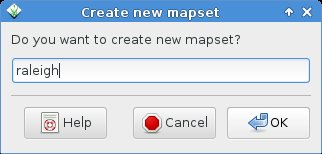
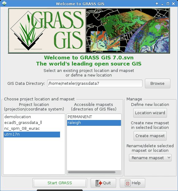
Now start GRASS GIS 7 and you will find the first band already imported (the others will follow shortly!).

For the lazy folks among us, we can also create a new GRASS GIS Location right away from the dataset on command line:

grass70 -c LC80160352013134LGN03_B10.TIF ~/grassdata/utm17n

Importing the remaining Landsat 8 bands

The remaining bands can be easily imported with the raster import tool:

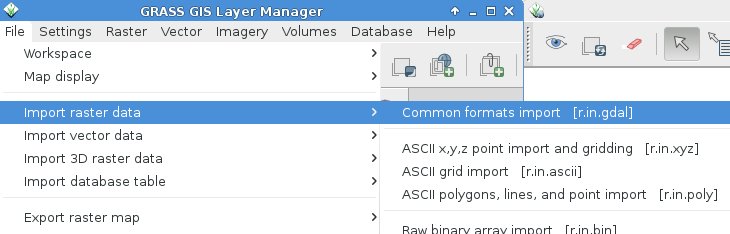
The bands can now be selected easily for import:

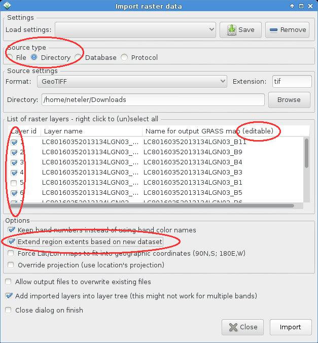
• Select “Directory” and navigate to the right one
• The available GeoTIFF files will be shown automatically
• Select those you want to import
• You may rename (double-click) the target name for each band
• Extend the computation region accordingly automatically

Click on “Import” to get the data into the GRASS GIS location. This takes a few minutes. Close the dialog window then.

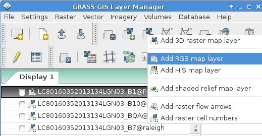
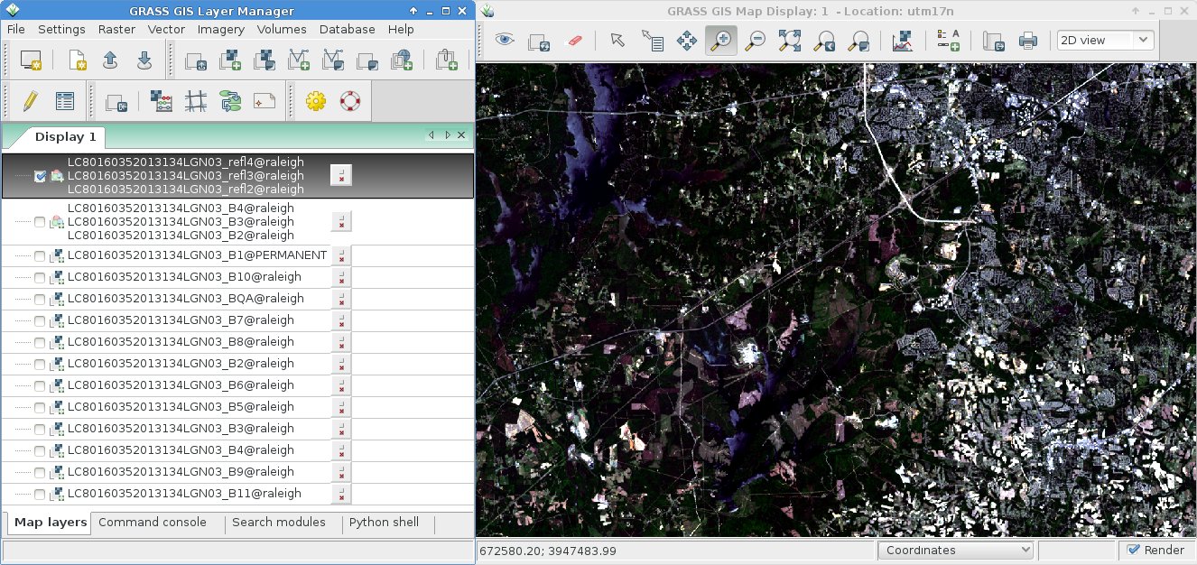
In the “Map layers” tab you can select the bands to be shown:

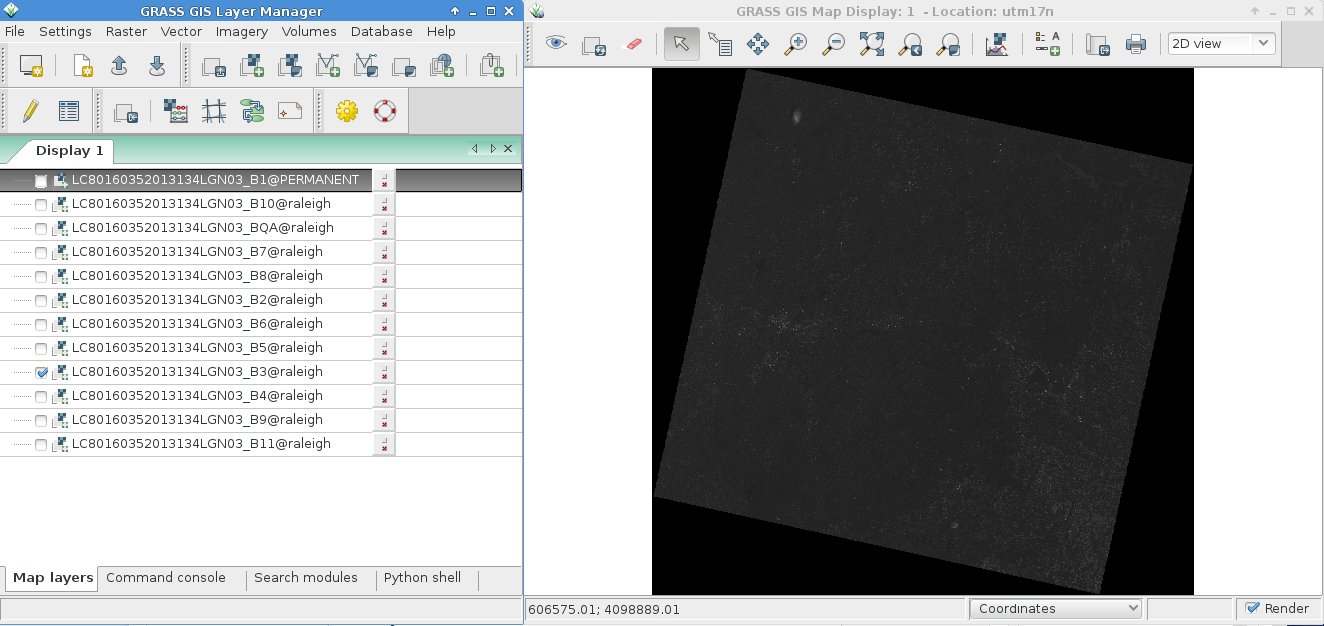
The bands of Landsat 8

(cited from USGS)

Landsat 8 Operational Land Imager (OLI) and Thermal Infrared Sensor (TIRS) images consist of nine spectral bands with a spatial resolution of 30 meters for Bands 1 to 7 and 9. New band 1 (ultra-blue) is useful for coastal and aerosol studies. New band 9 is useful for cirrus cloud detection. The resolution for Band 8 (panchromatic) is 15 meters. Thermal bands 10 and 11 are useful in providing more accurate surface temperatures and are collected at 100 meters. Approximate scene size is 170 km north-south by 183 km east-west (106 mi by 114 mi).

Landsat 7	Wavelength (micrometers)	Resolution (meters)		Landsat 8	Wavelength (micrometers)	Resolution (meters)
				Band 1 – Coastal aerosol	0.43 – 0.45	30
Band 1 – Blue	0.45 – 0.52	30		Band 2 – Blue	0.45 – 0.51	30
Band 2 – Green	0.52 – 0.60	30		Band 3 – Green	0.53 – 0.59	30
Band 3 – Red	0.63 – 0.69	30		Band 4 – Red	0.64 – 0.67	30
Band 4 (NIR)	0.77 – 0.90	30		Band 5 – Near Infrared (NIR)	0.85 – 0.88	30
Band 5 (SWIR 1)	1.55 – 1.75	30		Band 6 – SWIR 1	1.57 – 1.65	30
Band 7 (SWIR 2)	2.09 – 2.35	30		Band 7 – SWIR 2	2.11 – 2.29	30
Band 8 – Panchromatic	0.52 – 0.90	15		Band 8 – Panchromatic	0.50 – 0.68	15
				Band 9 – Cirrus	1.36- 1.38	30
Band 6 – Thermal Infrared (TIR)	10.40 -12.50	60* (30)		Band 10 – Thermal Infrared (TIRS) 1	10.60 – 11.19	100* (30)
				Band 11 – Thermal Infrared (TIRS) 2	11.50- 12.51	100* (30)
		* ETM+ Band 6 is acquired at 60-meter resolution. Products processed after February 25, 2010 are resampled to 30-meter pixels.				* TIRS bands are acquired at 100 meter resolution, but are resampled to 30 meter in delivered data product.

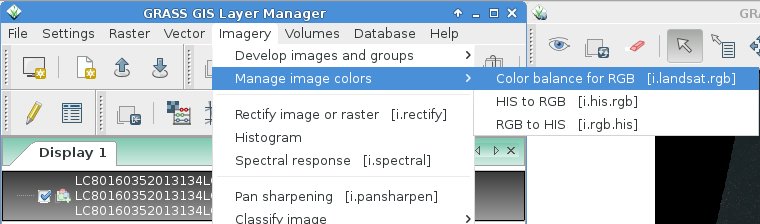
Natural color view (RGB composite)

Due to the introduction of a new “Cirrus” band (#1), the BGR bands are now 2, 3, and 4, respectively. See also “Common band combinations in RGB” for Landsat 7 or Landsat 5, and Landsat 8.

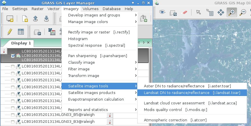
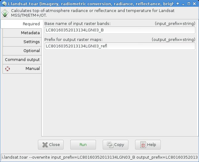
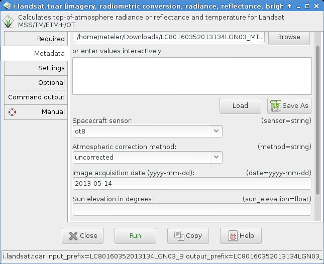
From Digital Numer (DN) to reflectance:
Before creating an RGB composite, it is important to convert the digital number data (DN) to reflectance (or optionally radiance). Otherwise the colors of a “natural” RGB composite do not look convincing but rather hazy (see background in the next screenshot). This conversion is easily done using the metadata file which is included in the data set with i.landsat.toar:

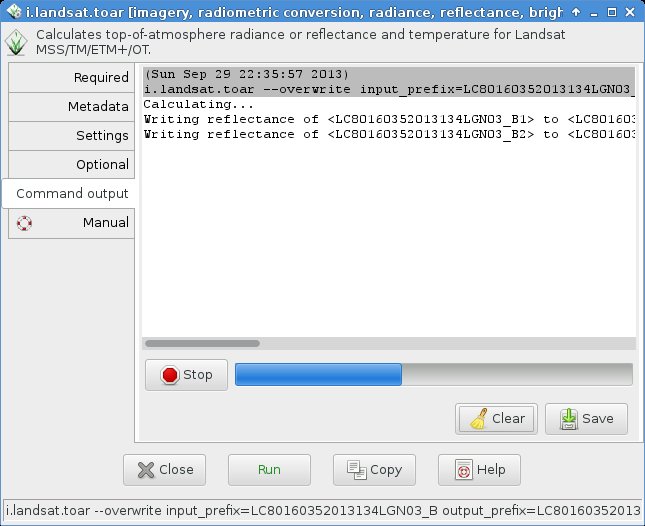
Now we are ready to create a nice RGB composite (hint 2015: i.landsat.rgb has been renamed to i.colors.enhance):

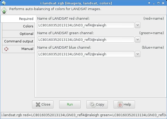
Select the bands to be visually combined:

… and voilà !

Applying the Landsat 8 Quality Assessment (QA) Band

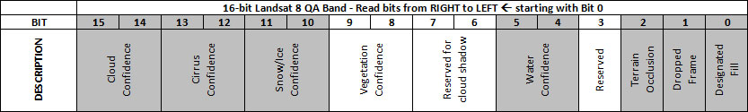
One of the bands of a Landsat 8 scene is named “BQA” which contains for each pixel a decimal value representing a bit-packed combination of surface, atmosphere, and sensor conditions found during the overpass. It can be used to judge the overall usefulness of a given pixel.

We can use this information to easily eliminate e.g. cloud contaminated pixels. In short, the QA concept is (cited here from the USGS page):

For the single bits (0, 1, 2, and 3):
0 = No, this condition does not exist
1 = Yes, this condition exists.

The double bits (4-5, 6-7, 8-9, 10-11, 12-13, and 14-15) represent levels of confidence that a condition exists:
00 = Algorithm did not determine the status of this condition
01 = Algorithm has low confidence that this condition exists (0-33 percent confidence)
10 = Algorithm has medium confidence that this condition exists (34-66 percent confidence)
11 = Algorithm has high confidence that this condition exists (67-100 percent confidence).

Detailed bit patterns (d: double bits; s: single bits):
d – Bit 15 = 0 = cloudy
d – Bit 14 = 0 = cloudy
d – Bit 13 = 0 = not a cirrus cloud
d – Bit 12 = 0 = not a cirrus cloud
d – Bit 11 = 0 = not snow/ice
d – Bit 10 = 0 = not snow/ice
d – Bit 9 = 0 = not populated
d – Bit 8 = 0 = not populated
d – Bit 7 = 0 = not populated
d – Bit 6 = 0 = not populated
d – Bit 5 = 0 = not water
d – Bit 4 = 0 = not water
s – Bit 3 = 0 = not populated
s – Bit 2 = 0 = not terrain occluded
s – Bit 1 = 0 = not a dropped frame
s – Bit 0 = 0 = not fill

Usage example 1: Creating a mask from a bitpattern

We can create a cloud mask (bit 15+14 are set) from this pattern:
cloud: 1100000000000000

Using the Python shell tab, we can easily convert this into the corresponding decimal number for r.mapcalc:

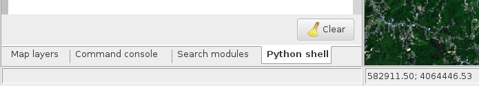
Welcome to wxGUI Interactive Python Shell 0.9.8

Type "help(grass)" for more GRASS scripting related information.
Type "AddLayer()" to add raster or vector to the layer tree.

Python 2.7.5 (default, Aug 22 2013, 09:31:58) 
[GCC 4.8.1 20130603 (Red Hat 4.8.1-1)] on linux2
Type "help", "copyright", "credits" or "license" for more information.
>>> int(0b1100000000000000)
49152

Using this decimal value of 49152, we can create a cloud mask:

# set NULL for cloudy pixels, 1 elsewhere:
r.mapcalc "cloudmask = if(LC80160352013134LGN03_BQA == 49152, null(), 1 )"

# apply this mask
r.mask cloudmask

In our sample scene, there are only tiny clouds in the north-east, so no much to be seen. Some spurious cloud pixels are scattered over the scene, too, which could be eliminated (in case of false positives) or kept.

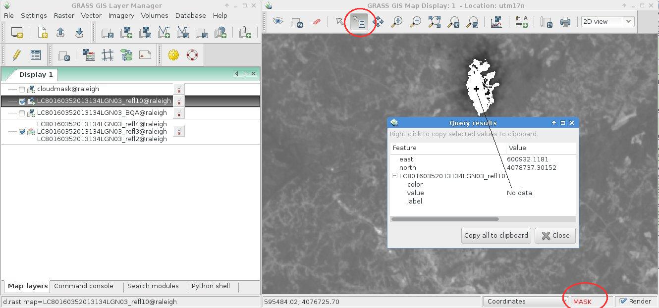
Usage example 2: Querying the Landsat 8 BQA map and retrieve the bitpattern

Perhaps you prefer to query the BQA map itself (overlay the previously created RGB composite and query the BSA map by selecting it in the Layer Manager). In our example, we query the BQA value of the cloud:

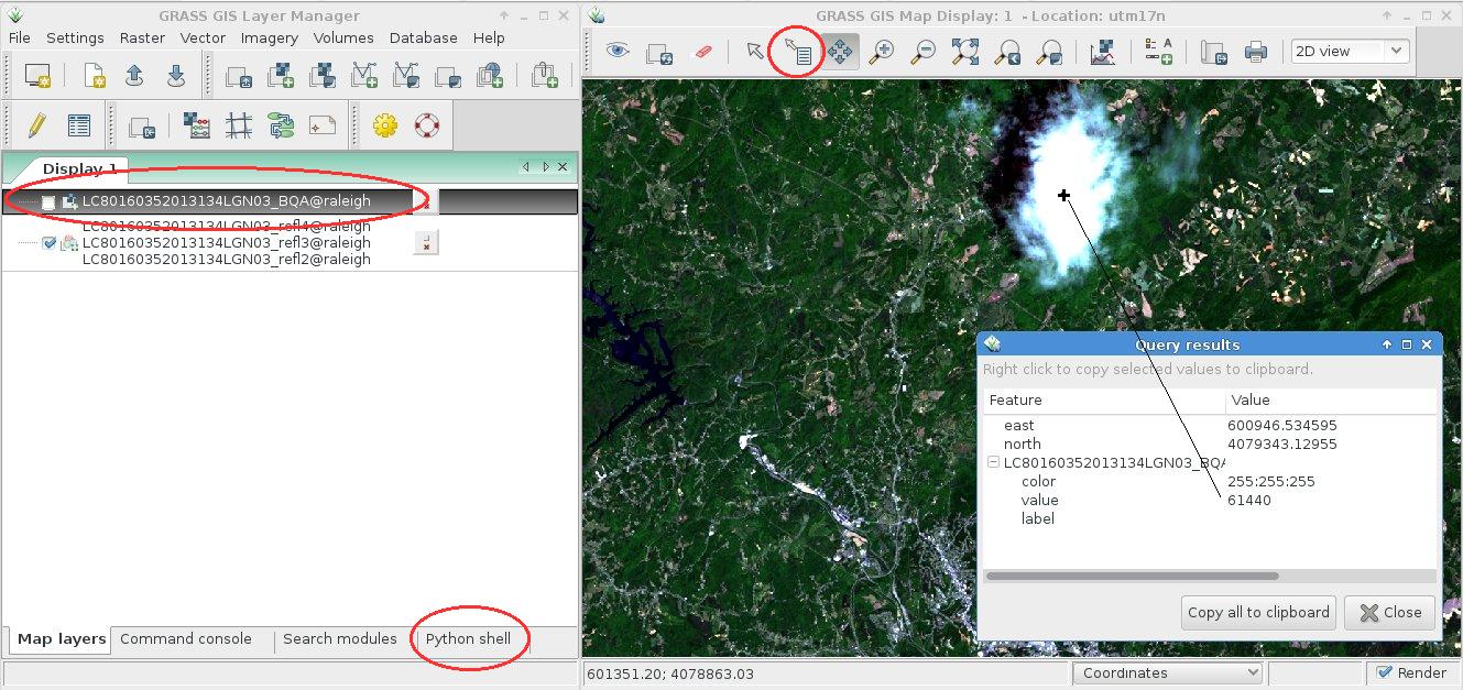
Using again the Python shell tab, we can easily convert the decimal number (used for r.mapcalc) into the corresponding binary representation to verify with the table values above.

>>> x=61440
>>> print(bin(x & 0xffffffff))
0b1111000000000000

Hence, bits 15,14,13, and 12 are set: cloudy and not a cirrus cloud. Looking at the RGB composite we tend to agree :-) Time to mask out the cloud!

wxGUI menu >> Raster >> Mask [r.mask]

Or use the command line, as shown already above:

# remove existing mask (if active)
r.mask -r

# set NULL for cloudy pixels, 1 elsewhere:
r.mapcalc "cloudmask = if(LC80160352013134LGN03_BQA == 61440, null(), 1 )" --o

# apply the new mask
r.mask cloudmask

The visual effect in the RGB composite is minimal since the cloud is white anyway (as NULL cells, too). However, it is relevant for real calculations such as NDVI (vegetation index) or thermal maps.

We observe dark pixels around the cloud originating from thin clouds. In a subsequent identification/mask step we may eliminate also those pixels with a subsequent filter.

See also Processing Landsat 8 data in GRASS GIS 7: RGB composites and pan sharpening