Importing and visualizing LAS LiDAR files in GRASS GIS 7: r.in.lidar

[toc]

LiDAR point cloud data are commonly delivered in the ASPRS LAS format. The format is supported by libLAS, a BSD-licensed C++ library for reading/writing these data. GRASS GIS 7 supports the LAS format directly when built against libLAS (as the case for most binary packages being available for download).

In this exercise we will import a sample LAS data set covering a tiny area close to Raleigh, NC (USA), belonging to the North Carolina sample data set. Sample LAS data download: https://grass.osgeo.org/sampledata/north_carolina/  (25MB).

For a full exercise, we will, however, assume that no GRASS GIS location is ready so far (so: newbies are welcome!) and create a new one initially.

1. Having the LAS file: now what?

In the first place, check the metadata of the LAS file using the lasinfo command (comes with libLAS; here only parts of the output shown):

lasinfo points.las
---------------------------------------------------------
  Header Summary
---------------------------------------------------------
  Version:  1.2
  Source ID:  0
  Reserved:  0
  Project ID/GUID:  '00000000-0000-0000-0000-000000000000'
  System ID:  'libLAS'
  Generating Software:  'libLAS 1.2'
[...]
  Spatial Reference:
None
[...]
---------------------------------------------------------
  Point Inspection Summary
---------------------------------------------------------
  Header Point Count: 1287775
  Actual Point Count: 1287775

  Minimum and Maximum Attributes (min,max)
---------------------------------------------------------
  Min X, Y, Z:   6066629.86, 2190053.45, -3.60
  Max X, Y, Z:   6070237.92, 2193507.74, 906.00
  Bounding Box:  6066629.86, 2190053.45, 6070237.92, 2193507.74
  Time:  0.000000, 0.000000
  Return Number:  1, 3
  Return Count:  1, 7
  Flightline Edge:  0, 0
  Intensity:  0, 256
  Scan Direction Flag:  0, 0
  Scan Angle Rank:  0, 0
  Classification:  2, 7
  Point Source Id:  0, 0
  User Data:  0, 0
  Minimum Color (RGB):  0 0 0 
  Maximum Color (RGB):  0 0 0 

  Number of Points by Return
---------------------------------------------------------
  (1) 1225886  (2) 61430  (3) 459

  Number of Returns by Pulse
---------------------------------------------------------
  (1) 30877  (2) 153  (5) 1225886  (6) 30706  (7) 153

  Point Classifications
---------------------------------------------------------
  647337 Ground (2) 
  639673 Low Vegetation (3) 
  740 Building (6) 
  25 Low Point (noise) (7) 
  -------------------------------------------------------
  0 withheld
  0 keypoint
  0 synthetic
  -------------------------------------------------------

We see: no spatial reference system indicated!
Luckily we know from here that the projection is  NAD83(HARN) / North Carolina, LCC 2SP metric, EPSG code 3358). Furthermore we see:

• Number of Points by Return: 3 (i.e., first, mid, last)
• Point Classifications: the points are already classified as “Ground” (class 2),  “Low Vegetation” (3),  “Building” (6), and Low Point (noise) (class 7). Something to play with later.

Time to create a GRASS GIS location and import the LAS file.

2. Creating a GRASS GIS location for the LAS file

Since we know the EPSG code of the projection, that’s an easy task. Please note that GRASS GIS can generate locations directly from SHAPE files (with .prj file), GeoTIFF and more.

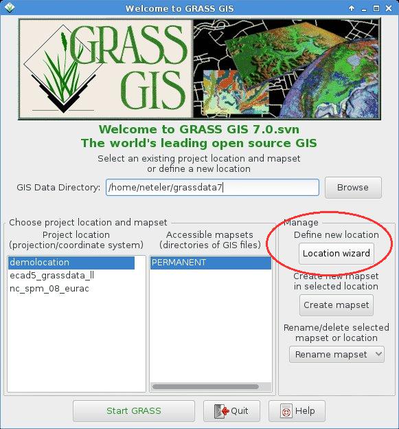
We fire up GRASS GIS 7 and open the Location Wizard:

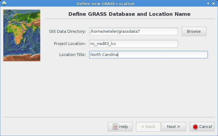
In the Location Wizard, we first define a name for the new location:

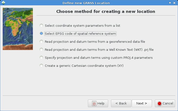
We select the “EPSG code” method for creating a new location:

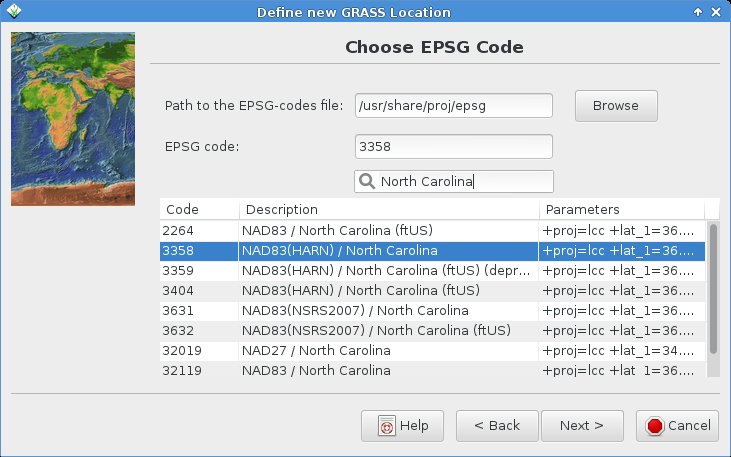
You can search for “North Carolina” and select the EPSG code 3358 from the list:

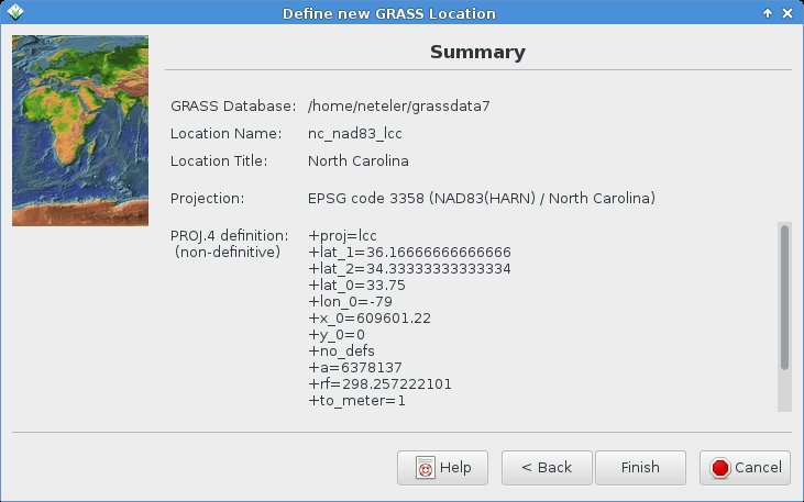
Next summary should show up as follows (be sure to have the metric projection shown!):

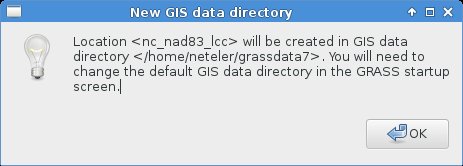
With “Finish” you reach this notification (indeed, nothing to change! It is already fine):

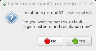
Since we want to import the LAS file, no need to manually define any region extent here – just say “No”:

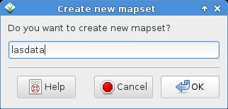
While we could import the data also into the PERMANENT mapset, we prefer to create an own mapset “lasdata” for our LAS data (once you reach hundreds of maps to manage, you will be happy about the concept of mapsets):

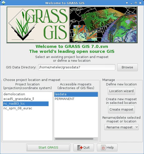
Voilà, we get back to the initial startup screen and can now start our GRASS GIS session with our “nc_nad83_lcc” location and “lasdata” mapset within the location: “Start GRASS”!

3. Import of the LAS file

When creating a new location from a GeoTIFF or SHAPE file (or other GDAL supported format), then the data set is imported right away. This is not the case for LAS files, also due to the fact that we can directly apply binning statistics during import of the LAS file (e.g. percentiles, min or max) and create a raster surface from the points right away rather than importing them as vector points.

3. a) Creating a raster surface from LAS during import

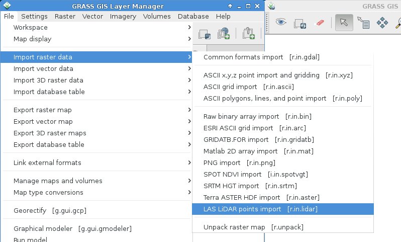
The LAS import into a raster surface is available through r.in.lidar:

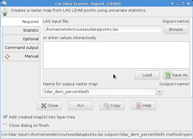
First the LAS file needs to be selected and an output file name specified (in this example, we want to extract the 95th percentile as binning method, hence a reasonable map name):

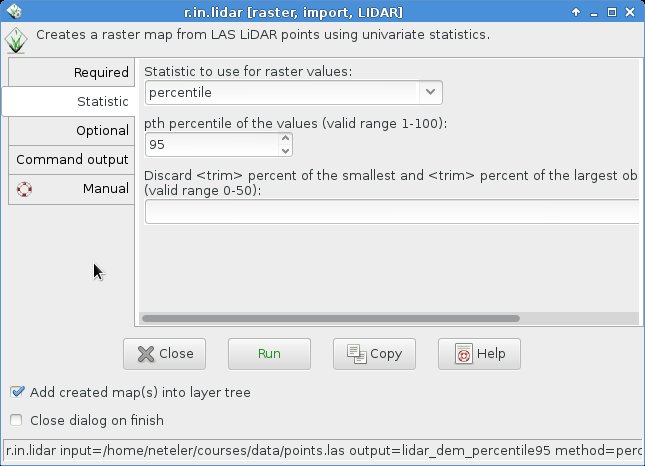
In the “Statistic” tab, we select the “percentile” method along with 95 as value:

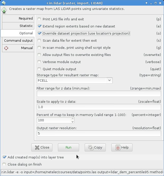
In the “Optional” tab we activate to extend the computational region from the LAS file and, since the spatial reference system metadata are lacking from the LAS file, also “override dataset projection” to use that predefined in the location. Finally, we define 5m as desired raster resolution for the resulting raster map:

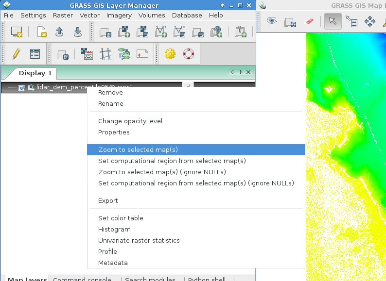
Upon conpletion of the import/binning, the new raster elevation map is shown after zooming to the map (r.in.lidar -e … restores upon completion the previous region settings, hence we may have to zoom):

Now we can start to analyze or visually explore the imported LAS file.

4. Visual LiDAR data exploration

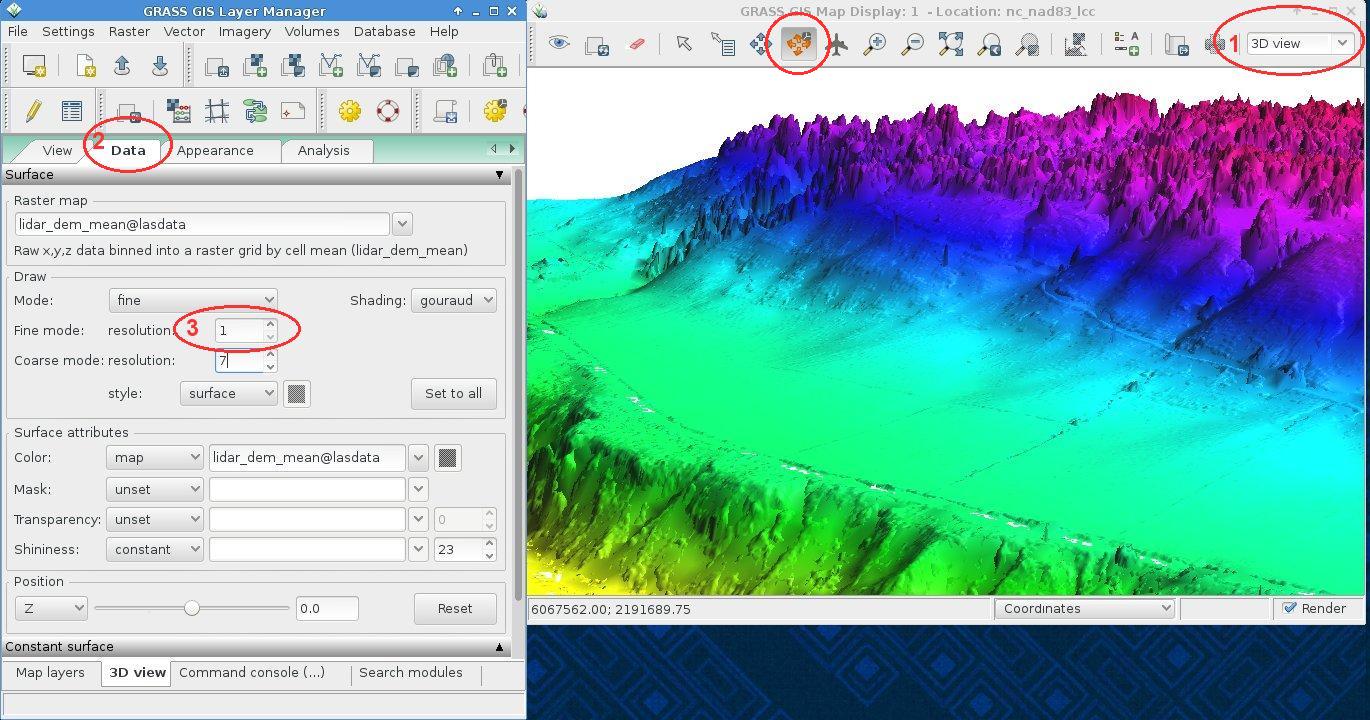
Using the wxNVIZ 3D viewer, we can easily fly through the new DEM. Switch in the Map Display to “3D view” (1). Note that the default rendering is initially done at low visual resolution for speed reasons. You can switch to “Rotate mode” as well to easily navigate with the mouse. In the “Data” tab (2) you can increase the visual resolution (3) to obtain a crisp view:

Now all kinds of analysis steps may follow.

Outlook

For true LiDAR processing as points, see the following GRASS GIS 7 modules: v.in.lidar (for point import), v.lidar.correction, v.lidar.edgedetection, v.lidar.growing, v.outlier, and v.surf.bspline.