Short Introduction to Geostatistical and Spatial Data Analysis with GRASS and R statistical data language

Learning statistical data analysis using "R"

1. Basics

R

R provides a set of base functions, which can be extended by using contributed packages (to be installed additionally).
Say, we needed such a contrib-package and therefore download and install the MASS library from Venable and Ripley. MASS provides many statistical functions and also numerous sample datasets:

#don't get confused: the code package is called VR, the library MASS:
install.packages("VR")
library(MASS)

To get R command help, you can always add a ? to the command:

?library
#or open the browser:
help.start()

Additionally there is the FAQ).
To get out of this (if already feeling sleepy):

q()

R is an object oriented data analysis language. The assignment operator is used to store results:

x <- 1+1

To get the result, just enter the name of the object:

x

Basics: Drawing a function

A simple example is to plot a sine curve. First we have to define the interval and number of data points to support the curve. Note: By redefining x we overwrite the old object:

x <- seq(-2*pi, 2*pi, len = 100)
x
str(x)
summary(x)

Then we can plot it (the type parameter specifies the line type):

matplot(x, sin(x), type="l")

To get an idea about the various "matplot()" options, run:

?matplot

You can see some "matplot()" examples by running:

example(matplot)

R comes along with a large number of published datasets. To get a list about currently accessible datasets, enter:

data()

To get a description of a specific dataset, enter (e.g. volcano dataset):

?volcano

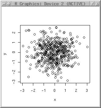
Before using such data, we generate a set of coordinate pairs (500 points) normally distributed (just to get some experience with R):

x <- rnorm(500)
y <- rnorm(500)

Plot them:

plot(x,y)

library(MASS)
truehist(x)
truehist(y, nbin=50)

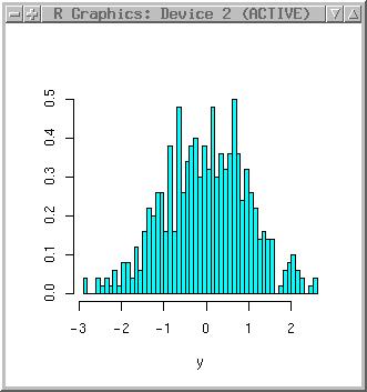
Let's add some z-values. To get numbers larger that 1 we multiply the values generated by rnorm:

z <- 1000 * rnorm(500)

To proceed, we need to link these three variables. They can be bounded into a "data frame":

dataset <- data.frame(x,y,z)

Now we have these variables twice, once individual, once in a dataframe. To see the objects currently available, use:

ls()

You can look at an object by entering its name. Here you will receive a long list of numbers with four columns (number of element, x, y, z):

dataset

Get a summary of it:

summary(dataset)

To look at the data structure (you will need to do this regularly), use the str() function:

str(dataset)

As we have a dataframe now, the access to a variable is different:

mean(x)

mean(dataset$x)

Hopefully you get the same results. Generally you could remove the individual variables if you will continue to work with the dataframe:

rm(x,y,z)
ls()

2. Visualization

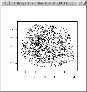
library(akima)
surface <- interp(dataset$x, dataset$y, dataset$z)
contour(surface)

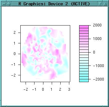
We want to see a colored surface with legend:

filled.contour(surface)

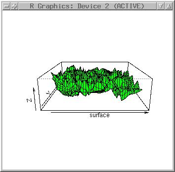
... and a perspective view:

persp(surface, col="green", expand=0.3)

New developments (2003) such as iPlots and RGL will improve the visualization capabilities of R. Also xyplot() of the lattice library is very powerful.

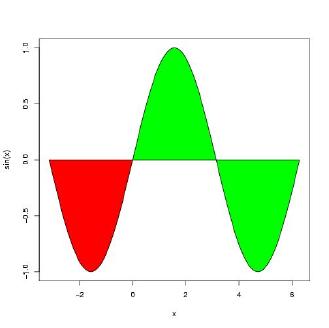
Finally we plot a color filled sine curve:

# set "frame":
plot(c(-pi, 2*pi), c(-1,1), type="n", ylab="sin(x)", xlab="x")
x1 <- seq(-pi, 0, length=101)
x2 <- seq(0, 2*pi, length=101)
polygon(c(0, -pi, x1), c(0, 0, sin(x1)), col="red")
polygon(c(2*pi, 0, x2), c(0, 0, sin(x2)), col="green")

# print plot into EPS file:
dev.copy2eps()

Import/export using ASCII-files (tables), manual table entry

x <- dataset$x

To export this single variable, use:

write(x, file="~/testfile.asc")

To export a dataframe, use:

write.table(dataset, file="~/testfile2.asc")

You probably want to use a column separator different from white space:

write.table(dataset, file="~/testfile3.asc", sep=":")

Read the table back into R:

dataset.new <- read.table("~/testfile.asc", header=T, sep=":")

Remove the x, y and z variable from memory of R (we still have the dataframe):

rm(x)

List available objects:

ls()

Now we want to get a summary of the dataframe variables (Min, 1st. Quartile, Median, Mean, 3rd Qu., Max, NA's):

summary(dataset)

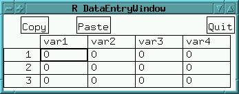
If you want to enter data tables from keyboard, R provides the function data.entry(). To enter a 3x4 matrix with value 0 pre-defining the fields, enter:

x <- matrix(0,3,4)
data.entry(x)

Plotting to file (EPS, PS)

postscript("test.ps")
plot(x)
dev.off()

xfig("test.fig")
plot(x)
dev.off()

dev.copy2eps()

Graphical user interface

# may not work on all systems:
install.packages("rgl", dependencies=TRUE)

# does not neccesarily need 'rgl':
install.packages("Rcmdr", dependencies=TRUE)

library(Rcmdr)

To re-lauch it, run:

Commander()

• Check that most of the menu items are greyed-out before a data set is read.
• Read the Prestige data set from the car package, via Data -> Data in packages -> Read data from an attached package.
• Test standard R graphics via Graphs -> Index plot, selecting income; then try a 3D plot of prestige vs. income and education; the 3D plot requires that the rgl package is installed.
• Fit a linear model, regressing prestige on education, income, and type, via Statistics -> Fit models -> Linear model.
• Test the linear hypothesis that the two coefficients for type are 0, via Models -> Hypothesis tests -> Linear hypothesis.
• Finally, test lattice graphics via Models -> Graphs -> Effect plots.

End of basic stuff.